Society for Political Methodology

By Tom Pepinsky

Valid instrumental variables are hard to find. The key identification assumption that an instrumental variable $Z$ be correlated with an endogenous variable $X$ , but not causally related to $Y$ , is difficult to justify in most empirical applications. Even worse, the latter of these requirements must be defended theoretically, it is untestable empirically. Recent concerns about “overfishing” of instrumental variables (Morck and Yeung 2011) underscore the severity of the problem. Every new argument that an instrumental variable is valid in one research context undermines the validity of that instrumental variable in other research contexts.

Given such challenges, it might be useful to consider more creative sources of instrumental variables that do not depend on any theoretical assumptions about how $Z$ affects $X$ or $Y$ . Given an endogenous variable $X$ , in a regression $Y = \beta X + u$ , why not simply generate random variables until we discover one that is, by happenstance, correlated with $X$ , and then use that variable $Z_{random}$ as an instrument? Because $Z_{random}$ is generated by the researcher, we can be absolutely certain that there is no theoretical channel through which it causes $Y$ . And because we have deliberately selected $Z_{random}$ so that it is highly correlated with $X$ , weak instrument problems should not exist. The result should be an instrument that is both valid and relevant. Right?

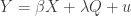
If it were only so easy. In Figure 1 below I show what would happen if we used random instruments, generated in the manner just described, for identification purposes. The data generating process, with notation following Sovey and Green (2011), is

$Y = \beta X + \lambda Q + u$
$X = \gamma Z + \delta Q + e$

$X$ is the endogenous variable, $Q$ is an exogenous control variable, and $Z$ is an instrumental variable. Endogenity arises from correlation between $u$ and $e$ , which are distributed multivariate standard normal with correlation $\rho = .5$ . For the simulations, $\beta=5$ , with $\lambda = \gamma = \delta = 1$ .

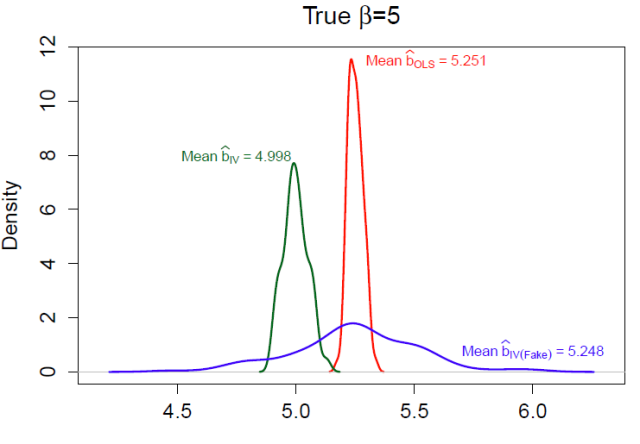
Figure 1: Random Instruments

Figure 1 shows the distribution of estimates $\hat{b}$ from 100 simulations of the data-generating process above. In each simulation, I generate each variable in Equations (1) and (2), and then repeatedly draw random variables until I happen upon one that is correlated with the randomly generated $X$ at the 99.9% confidence level. I use that variable $Z_{random}$ as an instrument to estimate $\hat{b}_{IV(Fake)}$ , which I compare to the naive OLS estimates $\hat{b}_{OLS}$ and estimates using the real instrument $Z$ from Equation (2), $\hat{b}_{IV}$ .

Clearly, OLS estimates are biased. But more importantly, the “fake” IV estimates are biased and inefficient, while “true” IV estimates using $Z$ are accurate. What has happened to the fake IVs?

How We Talk About Instruments

Understanding why this procedure fails to generate valid instruments requires a more precise understanding of the identification assumptions in instrumental variables regression than we normally find. The problem can be seen immediately in the introductory paragraph of this essay. My language followed common conventions in the ways that applied researchers talk about instrumental variables rather than the precise technical assumptions found in econometrics textbooks. I described the two requirements for instrumental variable as follows: an instrumental variable is some variable $Z$ that is

correlated with an endogenous variable $X$
not causally related to $Y$

These two statements are close, but not exact. The precise requirements (see e.g. Wooldridge 2002:83-84) are that $Z$ is

partially correlated with $X$ , conditional on $Q$ .
conditionally independent of $u$ , meaning that $\mathrm{Cov}[{Z,u}]=0$ .

Precision matters here. Assumption 1, usually referred to as the “relevance” of an instrument, emphasizes that $X$ and $Z$ must be partially correlated conditional on the exogenous variables $Q$ . The procedure described above simply looked for an unconditional correlation between $X$ and $Z$ , which may or may not suffice.

This is, however, a minor problem. We could follow Stock and Watson’s (2003: 350) advice, and search for variables $Z_{random}$ that satisfy the rule of thumb that the F statistic for a test that $\gamma=0$ in Equation (1) is greater than 10. The more fundamental assumption that prevents any type of randomized instrument from serving as a valid instrument for $X$ is the second assumption of “validity,” or that $\mathrm{Cov}[{Z,u}]=0$ .

This matters because $u$ is an unobservable quantity that reflects a theoretical claim about the data generating process that produces $Y$ . Consider what happens when we generate a $Z_{random}$ that is partially correlated with $X$ . $X$ is a function of $e$ , which is in turn correlated with $u$ —it is this correlation between $u$ and $e$ that motivates the instrumental variables approach to begin with. This chain of association $Z_{random} \rightarrow X \rightarrow e \rightarrow u$ makes it very likely that any $Z_{random}$ will also be correlated with $u$ , violating the assumption of validity. That chain of correlations from $Z$ to $u$ is what explains the biased and inefficient estimates for $\hat{b}_{IV(Fake)}$ in Figure 1.

Notice that not every $Z_{random}$ will be correlated with $u$ , but we can never know if any particular random instrument is. Consider would it would take to verify the validity of a random instrument. If we happened to observe the error term $u$ , then we could discard the majority of candidates for $Z_{random}$ that happened to also be correlated with $u$ , and select only valid random variables that happened to be partially correlated with $X$ and uncorrelated with $u$ . Figure 2 below shows two examples of binary $Z_{random}$ that are highly correlated with $X$ , but in the top case, $Z_{random}$ is also highly correlated with $u$ , whereas in the bottom case, $Z_{random}$ and $u$ are unrelated.

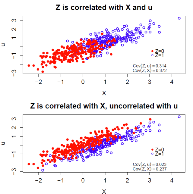
Figure 2: Comparing Z, X, and u

Again, if it were possible to observe $u$ , then it would be possible to choose only those instrumental variables $Z$ that were uncorrelated with $u$ . But the error term $u$ is unobservable by definition. So it is actually true that random instruments could work if we could check their correlation with $u$ , but since we cannot, the point is irrelevant in practice. Without access to $u$ , instrument validity is always a theoretical claim.

It is helpful to relate this conclusion about randomly generating instruments for observational data to randomized assignments to treatment offers in an experimental design with noncompliance. In such designs, assignment to treatment, or “intent to treat,” is an instrument for actual treatment. Here, randomization does ensure that the binary $Z$ is an instrument for treatment status $D$ , but only with appropriate assumptions about “compliers,” “never-takers,” “always takers,” and “defiers” (see Angrist, Imbens, and Rubin 1996). Gelman and Hill (2007) give the example of an encouragement design in which parents are randomly given inducements to expose their children to Sesame Street to test its effect on educational outcomes. If some highly motivated parents who would never expose their children to Sesame Street regardless of receiving the inducement or not (never-takers) use these inducements to “purchase other types of educational materials” (p. 218) that change their children’s educational outcomes, then the randomized inducement no longer estimates the average treatment effect among the compliers. The point is that randomizing treatment still requires the assumption that $\mathrm{Cov}[Z,u]=0$ , which in turn requires a model of $Y$ , for randomization to identify causal effects.

Precision, Insight, and Theory

How we as political scientists talk and write about instrumental variables almost certainly reflects how we think about them. In this way, casual, imprecise language can stand in the way of good research practice. I have used the case of random instruments to illustrate that we need to understand what would make an instrument valid in order to understand why we cannot just make them up. But there are other benefits as well to focusing explicitly on precise assumptions, with import outside of the fanciful world of thought experiments. To begin with, understanding the precise assumption $\mathrm{Cov}[Z,u]=0$ helps to reveal why all modern treatments emphasize that the assumption that $Z$ is a valid instrument is not empirically testable, but must be theoretically justified. It is not because we cannot think of all possible theories that link $Z$ to $Y$ . Rather, it is because because the assumption of validity depends on the relationship between the unobservable error term $u$ and any candidate instrument $Z$ .

Precision in talking and writing about instrumental variables will produce more convincing research designs. Rather than focusing on the relationship between $Y$ and $Z$ in justifying instrumental variables as source of identification, it may be more useful to focus instead on the empirical model of $Y$ . The most convincing identification assumptions are those that rest on a theory of the data-generating process for $Y$ to justify why $\mathrm{Cov}[Z,u]=0$ . Recalling that $u$ is not actually a variable, but might be better understood as a constructed model quantity, helps to emphasize that the theory that justifies the model of $Y$ is also the theory that determines the properties of $u$ . Indeed, without a model of the $Y$ it is hard to imagine how $u$ would relate to any particular instrument. A good rule of thumb, then, is no theory, no instrumental variables.

Thinking explicitly about $u$ rather than $Y$ and the model that it implies also helps to make sense of of what are sometimes called “conditional” instrumental variables. These are instruments whose validity depends on inclusion of an exogenous control variable (in the above example, $Q$ ) in the instrument variables setup. Conditional instruments are well understood theoretically: Brito and Pearl (2002) provide a framework for what they call “generalized” instrumental variables using directed acyclic graphs, and Chalak and White (2011) do the same in the treatment effects framework for what they call “extended” instrumental variables. Yet the imprecise short-hand description of the exclusion restriction as “ $Z$ is unrelated to $Y$ except through $X$ ” obscures these types of instruments. The observation that $u = Y - \beta X - \lambda Q$ immediately clarifies how control variables $Q$ can help with the identification of $\beta$ even if $X$ is still endogenous when controlling for $Q$ . Once again, a theory of the data generating process for $Y$ is instrumental for an argument about whether $Q$ can help to achieve identification.

Still another reason to pay close attention to the expression $\mathrm{Cov}[Z,u]$ is that it sheds light on how over identification tests work, and also on their limits. I have repeatedly stipulated that identification assumptions are not empirically testable, but it of course true that in an overidentified model with more instruments than endogenous variables, it is possible to reject the null hypothesis that all instruments are valid using a Hausman test. This test works by regressing the instruments $\bold{Z}$ and exogenous variable $Q$ on $\hat{u}$ , the two-stage least squares residuals when using $\bold{Z}$ as instruments for $X$ . With sample size $N$ , the product $N R_{\hat{u}}^2$ is asymptotically distributed $\chi_{K-1}^2$ , where $K \geq 2$ is the number of excluded instruments. Assuming homoskedasticity—there are alternative tests that are robust to heteroskedasticity—this provides a test statistic against the null that $\mathrm{Cov}[\bold{Z}',u]=0$ . It is true that a large test statistic rejects the null of overidentification, but small values for $N R_{\hat{u}}^2$ could have many sources: small $N$ , imprecise estimates, and others that have nothing to do with the “true” correlation between $\bold{Z}$ and $u$ . And even rejecting the null need not reject the validity of the instruments in the presence of treatment effect heterogeneity (see Angrist and Pischke:146).

Finally, a precise description of identification assumptions is important for pedagogical purposes. I doubt that many rigorous demonstrations of instrumental variables actually omit some discussion of the technical assumption that $\mathrm{Cov}[Z,u]=0$ , but this is presented in many different ways that, in my own experience, are confusing to students. Even two works from the same authors can differ! Take Angrist and Pischke, from Mastering ‘Metrics (2014): $Z$ must be “unrelated to the omitted variables that we might like to control for” (106). And from Mostly Harmless Econometrics (2009): $Z$ must be “uncorrelated with any other determinants of the dependent variable” (106). It is easy to see how these two statements may cause confusion, even among advanced students. Encouraging students to focus on the precise assumptions behind instrumental variables will help them to understand what exactly is at stake, both theoretically and empirically, when they encounter instrumental variables in their own work.

References

Angrist, Joshua D., Guido W. Imbens, and Donald B. Rubin (1996). “Identification of Causal Effects Using Instrumental Variables”. Journal of the American Statistical Association 91.434, pp. 444–455.

Angrist, Joshua D. and Jörn-Steffen Pischke (2009). Mostly Harmless Econometrics: An Empiricist’s Companion. Princeton: Princeton University Press.

— (2014). Mastering ‘Metrics: The Path from Cause to Effect. Princeton: Princeton University Press.

Brito, Carlos and Judea Pearl (2002). “Generalized Instrumental Variables”. In Uncertainty in Artificial Intelligence, Proceedings of the Eighteenth Conference. Ed. by A. Darwiche and N. Friedman. San Francisco.

Chalak, Karim and Halbert White (2011). “Viewpoint: An extended class of instrumental variables for the estimation of causal effects”. Canadian Journal of Economics 44.1, pp. 1–51.

Gelman, Andrew and Jennifer Hill (2007). Data Analysis Using Regression and Multilevel/Hierarchical Models. New York: Cambridge University Press.

Morck, Randall and Bernard Yeung (2011). “Economics, History, and Causation”. Business History Review 85 (1), pp. 39–63.

Sovey, Allison J. and Donald P. Green (2011). “Instrumental Variables Estimation in Political Science: A Readers’ Guide”. American Journal of Political Science 55 (1), pp. 188–200.

Stock, James H. and Mark W. Watson (2003). Introduction to Econometrics. New York: Prentice Hall.

Wooldridge, Jeffrey M. (2002). Econometric Analysis of Cross Section and Panel Data. Cambridge, MA: The MIT Press.

Why Can’t We Just Make Up Instrumental Variables?

How We Talk About Instruments

Precision, Insight, and Theory

References

Subscribe to our Mailing List