Understanding Equation Balance in Time Series Regression

By Peter K. Enns and Christopher Wlezien

Abstract: Most contributors to a recent Political Analysis symposium on time series analysis suggest that in order to maintain equation balance, one cannot combine stationary, integrated, and/or fractionally integrated variables with general error correction models (GECMs) and the equivalent autoregressive distributed lag (ADL) models. This definition of equation balance implicates most previous uses of these models in political science and circumscribes their use moving forward. The claim thus is of real consequence and worthy of empirical substantiation, which the contributors did not provide. Here we address the issue. First, we highlight the difference between estimating unbalanced equations and mixing orders of integration, the former of which clearly is a problem and the latter of which is not, at least not necessarily. Second, we assess some of the consequences of mixing orders of integration by conducting simulations using stationary and integrated time series. Our simulations show that with an appropriately speciﬁed model, regressing a stationary variable on an integrated one, or the reverse, does not increase the risk of spurious results. We then illustrate the potential importance of these conclusions with an applied example—income inequality in the United States.[1]

Political Analysis (PA) recently hosted a symposium on time series analysis that built upon De Boef and Keele’s (2008) inﬂuential time series article in the American Journal of Political Science. Equation balance was an important point of emphasis throughout the symposium. In their classic work on the subject, Banerjee, Dolado, Galbraith and Hendry (1993, 164) explain that an unbalanced equation is a regression, “in which the regressand is not the same order of integration as the regressors, or any linear combination of the regressors.” The contributors to this symposium were right to emphasize the importance of equation balance, as unbalanced equations can produce serially correlated residuals (e.g., Pagan and Wickens 1989) and spurious relationships (e.g., Banerjee et al. 1993, 79).

Throughout the PA symposium, however, equation balance is deﬁned and applied in different ways. Grant and Lebo (2016, 7) follow Banerjee, et al’s deﬁnition when they explain that a general error correction model (GECM)—or autoregressive distributed lag (ADL)—is balanced if co-integration is present.[2] Keele, Linn and Webb (2016a, 83) implicitly make this same point in their second contribution to the symposium when they cite Bannerjee et al. (1993) in their discussion of equation balance. Yet, other parts of the symposium seem to apply a stricter standard of equation balance, stating that when estimating a GECM/ADL all time series must be the same order of integration. As Grant and Lebo write in the abstract of their ﬁrst article, “Time series of various orders of integration—stationary, non-stationary, explosive, near-and fractionally integrated—should not be analyzed together… That is, without equation balance the model is misspecified and hypothesis tests and longrun-multipliers are unreliable.” Keele, Linn and Webb (2016b, 34) similarly write, “no regression model is appropriate when the orders of integration are mixed because no long-run relationship can exist when the equation is unbalanced.” Box-Steffensmeier and Helgason (2016, 2) make the point by stating, “when studying the relationship between two (or more) series, the analyst must ensure that they are of the same level of integration; that is, they have to be balanced.” Although Freeman (2016) offers a more nuanced perspective on equation balance, many of the symposium contributors could be interpreted as recommending that scholars never mix orders of integration.[3] Indeed, in their concluding article, Lebo and Grant write, “One point of agreement among the papers here is that equation balance is an important and neglected topic. One cannot mix together stationary, unit-root, and fractionally integrated variables in either the GECM or the ADL” (p.79).

It is possible that these authors did not mean for these quotes to be taken literally. However, we both have recently been asked to review articles that have used these quotes to justify analytic decisions with time series data.[4] Thus, we think the claims should be reviewed carefully. This is especially the case because Grant and Lebo could be interpreted as applying these strict standards in some of their empirical applications. For example, in their discussion of Sánchez Urribarrí, Schorpp, Randazzo and Songer (2011), Grant and Lebo write, “both the UK and US models are unbalanced—each DV is stationary, and the inclusion of unit-root IVs has compromised the results” (Supplementary Materials, p.36). Researchers might take this statement to imply that including stationary and unit root variables automatically produces an unbalanced equation.

In addition to holding implications for practitioners, the strict interpretation of equation balance holds implications for the vast number of existing time series articles that employ GECM/ADL models without pre–whitening the data to ensure equal orders of integration across all series. Lebo and Grant (2016, 79) point out, for example, “FI [fractional integration] methods allow us to create a balanced equation from dissimilar data. By ﬁltering each series by its own (p, d, q) noise model, the residuals of each can be rendered (0, 0, 0) so that you can investigate how X’s deviations from its own time-dependent patterns affect Y’s deviations from its own time-dependent patterns.” Fortunately, existing time series analysis that does not pre-whiten the data need not be automatically dismissed. The strict interpretation of equation balance—i.e., that mixing orders of integration is always problematic with the GECM/ADL—is not accurate. As noted above, the contributors to the symposium may indeed understand this point. But based on the quotes above, we feel that it is important to clarify for practitioners that an unbalanced equation is not synonymous with mixing orders of integration. While related, they are not the same, and while the former is always a problem the latter is not.

We begin by showing that equation balance does not necessarily require that all series have the same order of integration with the GECM/ADL. This is important because the classic examples in the literature of unbalanced equations include series of different orders of integration (see, for example, Banerjee et al. (1993, 79) and Maddala and Kim (1998, 252)). But our results are not at odds with these scholars, as their examples all assume a relationship with no dynamics. When using a GECM/ADL to model dynamic processes, even mixed orders of integration can produce balanced equations. This conclusion is consistent with Banerjee et al. (1993), who write, “The moral of the econometricians’ story is the need to keep track of the orders of integration on both sides of the regression equation, which usually means incorporating dynamics; models that have restrictive dynamic structures are relatively likely to give misleading inferences simply for reasons of inconsistency of orders of integration” (p.192, italics ours).

We believe the PA symposium was not suﬃciently clear that adding dynamics can solve the equation balance problem with mixed orders of integration. Thus, a key contribution of our article is to show how appropriate model speciﬁcation can be used to produce equation balance and avoid inﬂating the rate of spurious regression—even when the model includes series with different orders of integration. Our particular focus is analysis that mixes stationary I(0) and integrated I(1) time series. In practice, researchers might encounter other types of time series, such as fractionally integrated, near-integrated, or explosive series. Evaluating every type of time series and the vast number of ways different orders of integration could appear in a regression model is beyond the scope of this paper. Our goal is more basic, but still important. We aim to demonstrate that there are exceptions to the claim that, “The order of integration needs to be consistent across all series in a model” (Grant and Lebo 2016, 4) and that these exceptions can hold important implications for social science research.

More speciﬁcally, we show that when data are either stationary or (ﬁrst order) integrated, scenarios exist when a GECM/ADL that includes both types of series can be estimated without problem. Our simulations show that regressing an integrated variable on a stationary one (or the reverse) does not increase the risk of spurious results when modeled correctly. While this may be a simple point, we think it is a crucial one. As mentioned above, if readers interpreted the previous quotes from the PA symposium as deﬁning equation balance to mean that different orders of integration cannot be mixed, most existing research that employs the ADL/GECM model would be called into question. Given the fact that Political Analysis is one of the most cited journals in political science and the symposium included some of the top time series practitioners in the discipline, we believe it is valuable to clarify that mixing orders of integration is not always a problem and that existing time series research is not inherently ﬂawed. Furthermore, the one article that has responded to particular claims made in the symposium contribution did not address the symposium’s deﬁnition of equation balance (Enns et al. 2016).[5] We hope our article helps clarify the concept of equation balance for those who use time series analysis.

We also illustrate the importance of our ﬁndings with an applied example—income inequality in the United States. The example illustrates how the use of pre-whitening to force variables to be of equal orders of integration (when the equation is already balanced) can be quite costly, leading researchers to fail to detect relationships.[6]

Clarifying Equation Balance

The contributors to the PA symposium were all correct to emphasize equation balance. Time series analysis requires a balanced equation. An unbalanced equation is mis-speciﬁed by deﬁnition, typically resulting in serially correlated residuals and an increased probability of Type I errors.[7] As noted above, Banerjee et al. (1993, 164, italics ours) explain that an unbalanced equation is a regression, “in which the regressand is not the same order of integration as the regressors, or any linear combination of the regressors.” Our primary concern is that much of the discussion in the PA symposium seems to focus on the order of integration of each variable in the equation without acknowledging that a “linear combination of the regressors” can also produce equation balance. We worry that researchers might interpret this focus to mean that equation balance requires each series in the model to be the same order of integration.[8] Such a conclusion would be wrong. As the previous quote from Banerjee et al. (1993) indicates (also see, Maddala and Kim (1998, 251), if the regressand and the regressors are not the same order of integration, the equation will still be balanced if a linear combination of the variables is the same order of integration.

As Grant and Lebo (2016, 7) and Keele, Linn and Webb (2016a, 83) acknowledge, cointegration offers a useful illustration of how an equation can be balanced even when the regressand and regressors are not the same order of integration.[9] Consider two integrated I(1) variables, Y and X, in a standard GECM model:

$\Delta Y_t = \alpha_0 + \alpha_1 Y_{t-1} + \gamma_1 \Delta X_t + \beta_1 X_{t-1} + \epsilon_t.$ (1)

Clearly, the equation mixes orders of integration. We have a stationary regressand ( $\Delta Y_t$ ) and a combination of integrated ( $Y_{t-1}$ , $X_{t-1}$) and stationary ( $\Delta X_t$ ) regressors. However, if X and Y are cointegrated, the equation is still balanced. To see why, we can rewrite Equation 1 as:

$\Delta Y_t = \alpha_0 + \alpha_1 (Y_{t-1} + \frac{\beta_1}{\alpha_1} X_{t-1}) + \gamma_1 \Delta X_{t} + \epsilon_t.$ (2)

X and Y are cointegrated when X and Y are both integrated (of the same order) and $\alpha_1$ and and $\beta_1$ are non-zero (and $\alpha_1$ Y and X maintain an equilibrium relationship, a linear combination of these variables exists that is stationary (that is, if we regress Y on X, in levels, the residuals would be stationary).[10] As noted above, this (stationary) linear combination is captured by $(Y_{t-1} + \frac{\beta_1}{\alpha_1}X_{t-1})$ . Additionally, since Y and X are both integrated of order one, $\Delta Y$ and $\Delta X$ will be stationary. Thus, cointegration ensures that the equation is balanced: the regressand ( $\Delta Y_t$ ) and either the regressors ( $\Delta X_t$ ) or a linear combination of the regressors $(Y_{t-1} + \frac{\beta_1}{\alpha_1}X_{t-1})$ are all stationary. Importantly, if we added a stationary regressor to the model, e.g., if we thought innovations in Y were also inﬂuenced by a stationary variable, the equation would still be balanced.

The fact that the GECM—which mixes stationary and integrated regressand and regressors—is appropriate when cointegration is present demonstrates that equation balance does not require the series to be the same order of integration. As we have mentioned, Grant and Lebo (2016, 7) acknowledge that a GECM is balanced if co-integration is present and Keele, Linn and Webb (2016a, 83) make this point in their second contribution to the symposium citing Bannerjee et al. (1993) in their discussion of equation balance. However, as noted above, we have begun to encounter research that interprets other statements in the symposium to mean that analysts can never mix orders of integration. For example, in their discussion of Volscho and Kelly (2012), Grant and Lebo write that the “data is a mix of data types (stationary and integrated), so any hypothesis tests will be based on unbalanced equations” (supplementary appendix, p. 48). But is this this really the case? The above example shows that when cointegration is present, equation balance can exist even when the orders of integration are mixed.

Below, we use simulations to illustrate two seemingly less well-known scenarios when equation balance exists despite different orders of integration. Again, our goal is not to identify all cases where different orders of integration can result in equation balance. Rather, we want to show that researchers should not automatically equate different orders of integration with an unbalanced equation. Situations exist where it is completely appropriate to estimate models with different orders of integration.

Equation Balance with Mixed Orders of Integration: Simulation Results

We begin with an integrated Y and a stationary X. At ﬁrst glance, estimating a relationship between these variables, which requires mixing an I(1) and I(0) series, might seem problematic. Grant and Lebo (2016, 4) explain, “Mixing together series of various orders of integration will mean a model is misspecified” and in econometric texts, mixing I(1) and I(0) series offers a classic example of an unbalanced equation (Banerjee et al. 1993, 79, Maddala and Kim 1998, 252).[11]

It is still possible to estimate the relationship between an integrated Y and a stationary X in a correctly speciﬁed and balanced equation. First, we must recognize that when Banerjee et al. (1993) (see also Mankiw and Shapiro (1986) and Maddala and Kim (1998)) state that an I(1) and I(0) series represent an unbalanced equation, they are modeling the equation:

$y_t = \alpha + \beta x_{t-1} + u_t.$ (3)

Equation 3 is indeed unbalanced (and thus misspecified) as the regressand is integrated and the regressor is stationary. This result does not, however, mean that we cannot consider these two series. A stationary series, X, might be related to innovations in an integrated series, Y. If so, we could model this process with an autoregressive distributed lag model:

$Y_t = \alpha + \alpha_1 Y_{t-1} + \beta_1 X_t + \beta_2 X_{t-1} + \epsilon.$ (4)

Much as before, this might appear to still be an unbalanced equation. We continue to mix I(1) and I(0) series, which seemingly violates Lebo and Grant’s (2016, 71) conclusion that, “One cannot mix together stationary, unit–root, and fractionally integrated variables in either the GECM or the ADL.”[12] However, since Y is I(1), $\alpha_1$ = 1, which means $Y_t - \alpha_1 Y_{t-1} = \Delta Y$ . Thus, we can rewrite the equation as,

$\Delta Y_t = \alpha + \beta_1 X_t + \beta_2 X_{t-1} + \epsilon.$ (5)

Because Y is an integrated, I(1), series, $\Delta Y$ must be stationary. Thus, the regressand and regressors are all I(0) series. As Banerjee et al. (1993, 169) explain, “regressions that are linear transformations of each other have identical statistical properties. What is important, therefore, is the possibility of transforming in such a way that the regressors are integrated of the same order as the regressand.”[13] Thus, Equation 5 shows that the ADL in Equation 4 is indeed balanced. (Because the GECM is algebraically equivalent to the ADL, the GECM would—by denition—also be balanced in this example.)

The above discussion suggests that we can use an ADL to estimate the relationship between an integrated Y and stationary X. To test these expectations, we conduct a series of Monte Carlo experiments. We generate an integrated Y with the following DGP:

$Y_t= Y_{t-1} + \epsilon_{yt},\; \epsilon_{yt}\sim N(0,1).$ (6)

We generate the stationary time series X, with the following DGP, where $\theta$ equals 0.0 or 0.5:

$X_t=\theta_x X_{t-1} + \epsilon_{xt},\; \epsilon_{xt}\sim N(0,1).$ (7)

Notice that X and Y are independent series. Particularly with dependent series that contain a unit root (as is the case here), the dominant concern in time series literature is the potential for estimating spurious relationships (e.g., Granger and Newbold 1974, Grant and Lebo 2016, Yule 1926). Thus, our ﬁrst simulations seek to identify the percentage of analyses that would incorrectly reject the null hypothesis of no relationship between a stationary X and integrated Y with an ADL. As noted above, in light of the recommendations in the PA symposium to never mix orders of integration, this approach seems highly problematic. However, if the equation is balanced as we suggest, the false rejection rate in our simulations should only be about 5 percent.

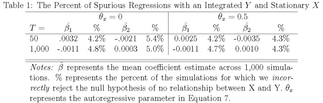
In the following simulations, T is set to 50 and then 1,000. These values allow us to evaluate both a short time series that political scientists often encounter and a long time series that will approximate the asymptotic properties of the series. We use the DGP from Equations 6 and 7, above, to generate 1,000 simulated data sets. Recall that in our stationary series, $\theta_x$ equals 0.5 or 0.0 and Y and X are never related. To evaluate the relationship between X and Y, we estimate an ADL model in Equation 4.[14]

EnnsWlezienTable1

Table 1 reports the average estimated relationship across all simulations between X and Y ( $\hat{\beta_1}$ and $\hat{\beta_2}$ in Equation 4) and the percent of simulations in which these relationships were statistically signiﬁcant. The mean estimated relationship is close to zero and the Type I error rate is close to 5 percent. With this ADL speciﬁcation, when Y is integrated and X is stationary, mixing integrated and stationary time series does not increase the risk of spurious regression.[15]

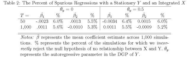
Results in Table 2 show that the same pattern of results emerges when X is integrated and Y is stationary.[16] Most time series analysis in the political and social sciences could be accused of mixing orders of integration. Thus, the recommendations of the PA symposium could be interpreted as calling this research into question. We have shown, however, that mixing orders of integration does not automatically imply an unbalanced equation. It also does not automatically lead to spurious results.

The Rise of the Super Rich: Reconsidering Volscho and Kelly (2012)

We think the foregoing discussion and analyses offer compelling evidence that, despite the range of statements about equation balance in the PA symposium, mixing orders of integration when using a GECM/ADL does not automatically pose a problem to researchers. Of course, to a large degree the previous sections reiterate and unpack what econometricians have shown mathematically (e.g., Sims, Stock and Watson 1990), and so may come as little surprise to some readers (especially those who have not read the PA Symposium). Here, we use an applied example to illustrate the importance of correctly understanding equation balance. We turn to a recent article by Volscho and Kelly (2012) that analyzes the rapid income growth among the super-rich in the United States (US). They estimate a GECM of pre-tax income growth among the top 1% and ﬁnd evidence that political, policy, and economic variables inﬂuence the proportion of income going those at the top. Critically for our purposes, they include stationary and integrated variables on the right-hand side, which Grant and Lebo (2016, 26) actually single out as a case where the “GECM model [is] inappropriate with mixed orders of integration.” Grant and Lebo go on to assert that Volscho and Kelly’s “data is a mix of data types (stationary and integrated), so any hypothesis tests will be based on unbalanced equations” (supplementary appendix, p. 48). Based on the conclusion that mixing orders of integration produces an unbalanced equation, Grant and Lebo employ fractional error correction technology and find that none of the political or and policy variables (and only some economic variables) matter for incomes among the top 1%.

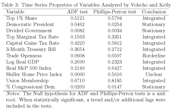
These are very different ﬁndings, ones with potential policy consequences, and so it is important to reconsider what Volscho and Kelly did—and whether the mixed orders of integration pose a problem for their analysis. To begin our analysis, we present the dependent variable from Voschlo and Kelly, the total pre-tax income share of the top 1% for the period between 1913 and 2008.[17] In Figure 1 we can see that income shares start off quite high and then drop and then return to inter-war levels toward the end of the series. The variable thus exhibits none of the trademarks of a stationary series, i.e., it is not mean-reverting, and looks to contain a unit root instead. Notice that the same is true for the shorter period encompassed by Volscho and Kelly’s analysis, 1949-2008. Augmented Dickey-Fuller (ADF) and Phillips–Perron unit root tests conﬁrm these suspicions, and are summarized in the ﬁrst row of Table 3, below.[18]

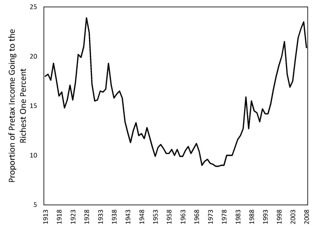
Figure 1: The Top 1 Percent’s Share of Pre-tax Income in the United States, 1913 to 2008

What about the independent variables? Here, we ﬁnd a mix (see Table 3). Some variables clearly are nonstationary and also appear to contain unit roots: the capital gains tax rate, union membership, the Treasury Bill rate, Gross Domestic Product (logged), and the Standard and Poor 500 composite index. The top marginal tax rate also is clearly nonstationary and we cannot reject a unit root even when taking into account the secular (trending) decline over time. The results for the Shiller Home Price Index are mixed and trade openness is on the statistical cusp, and there is reason—based on the size of the autoregressive parameter (-0.29) and the fact that we reject the unit root over a longer stretch of time—to assume that the variable is stationary. For the other variables included in the analysis, we reject the null hypothesis of a unit root: Democratic president, and the Percentage of Democrats in Congress. These ﬁndings seem to comport with what Volscho and Kelly found (see their supplementary materials).[19]

EnnsWlezienTable3

Volscho and Kelly proceed to estimate a GECM of the top 1% income share including current ﬁrst differences and lagged levels of the stationary and integrated variables. So far, the diagnostics support their decision (integrated DV, some IVs are integrated, and we ﬁnd evidence of cointegration).[20] The fact that stationary variables are also included in the model should not affect equation balance. However, in order to evaluate the robustness of Volscho and Kelly’s results, we re-consider their data with Pesaran and Shin’s ARDL (Autoregressive Distributed Lag) critical bounds testing approach (Pesaran, Shin and Smith 2001). Although political scientists typically refer to the autoregressive distributed lag model as an ADL, Pesaran, Shin and Smith (2001) prefer ARDL. For their bounds test of cointegration, they estimate the model as a GECM.[21]

The ARDL approach is one of the approaches recommended by Grant and Lebo and is especially advantageous in the current context because two critical values are provided, one which assumes all stationary regressors and one which assumes all integrated regressors. Values in between these “bounds” correspond to a mix of integrated and stationary regressors, meaning the bounds approach is especially appropriate when the analysis includes both types of regressors. Grant and Lebo (2016, 19) correctly acknowledge that “With the bounds testing approach, the regressors can be of mixed orders of integration—stationary, non-stationary, or fractionally integrated—and the use of bounds allow the researcher to make inferences even when the integration of the regressors is unknown or uncertain.”[22] Since Table 3 indicates we have a mix of stationary and integrated regressors, if our critical value exceeds the highest bound, we will have evidence of cointegration.

The ARDL approach proceeds in several steps.[23] First, if the dependent variable is integrated, the ARDL model (which is equivalent to the GECM) is estimated. Next, if the residuals from this model are stationary, an F-test is conducted to evaluate the null hypothesis that the combined effect of all lagged variables in the model equals zero. This F statistic is compared to the appropriate critical values (Pesaran, Shin and Smith 2001). We rely on the small-sample critical values from Narayan (2005). If there is evidence of cointegration, both long and short-run relationships from the initial ARDL (i.e., ADL/GECM) model can be evaluated.

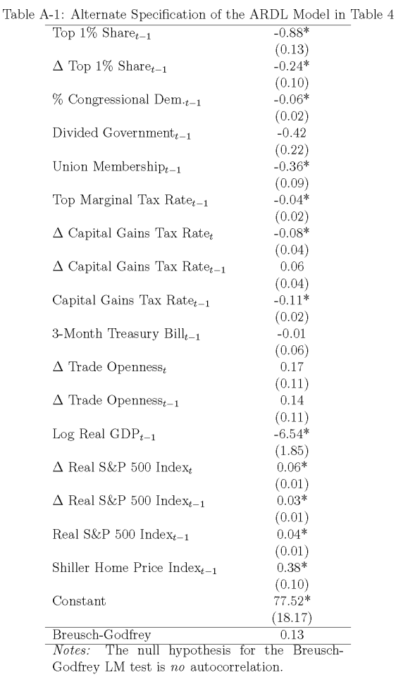
Our analysis focuses on Column 5 from Volscho and Kelly’s Table 1, which is their preferred model. The ﬁrst column of our Table 4, below, shows that we successfully replicate their results. The ARDL analysis appears in Column 2.[24] The key difference between this specication and that of Volscho and Kelly’s is that they (based on a Breusch-Godfrey test) employed the Prais-Winsten estimator to correct for serially correlated errors and we do not. Our decision reﬂects the fact that other tests do not reject the null of white noise, e.g., the Portmanteau (Q) test produces a p-value of 0.12, and it allows us to compare the results with and without the correction. Also note that an expanded model including lagged differenced dependent and independent variables (see Appendix Table A-1) produces very similar estimates to those shown in column 2 of Table 4, and a Breusch-Godfrey test indicates that the resulting residuals are uncorrelated.

To begin with, we need to test for cointegration. For this, we compare the F-statistic from the lagged variables (6.54) with the Narayan (2005) upper (I(1)) critical value (3.82), which provides evidence of cointegration.[25] The Bounds t-test also supports this inference, as the t-statistic (-7.75) for the $Y_{t-1}$ parameter is greater (in absolute terms) than the I(1) bound tabulated by Pesaran, Shin, and Smith (2001, 303). Returning to the results in Column 2, we see that the ARDL approach produces similar conclusions to Column 1. (Philips (2016) uses the ARDL approach to re-consider the ﬁrst model in Volscho and Kelly’s (2012) Table 1 and also obtains similar results.) The coefficients for all but two of the independent variables have similar effects, i.e., the same sign and statistical signiﬁcance.[26] The exceptions are Divided Government_(t-1) and $\Delta$ Trade Openness, for which the coeﬃcients using the two approaches are similar but the standard errors differ substantially. Consistent with the existing research on the subject, we ﬁnd evidence that economics, politics, and policy matter for the share of income going to the top 1 percent.

EnnsWlezienTable4

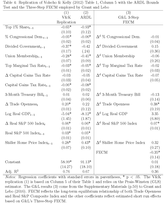
Although Grant and Lebo (2016, 18) recommend both the ARDL approach and a three-step fractional error correction model (FECM) approach, they only report the results for the latter in their re-analysis of Volscho and Kelly.[27] It turns out that the two approaches produce very different results. This can be seen in column 3 of Table 4, which reports Grant and Lebo’s FECM reanalysis of Volscho and Kelly Model 5 (from Grant and Lebo’s supplementary appendix, p. 50). With their approach, only the change in stock prices (Real S&P 500 Index) and Trade Openness are statistically signiﬁcant (p.05 predictors="" of="" income="" shares="" though="" levels="" stock="" prices="" and="" trade="" openness="" also="" matter="" via="" the="" fecm="" component="" which="" captures="" disequilibria="" between="" those="" variables="" lagged="" shares.="" despite="" theoretical="" empirical="" evidence="" suggesting="" that="" marginal="" tax="" rate="" piketty="" saez="" stantcheva="" union="" strength="" myers="" pontusson="" western="" rosenfeld="" partisan="" composition="" government="" hibbs="" kelly="" can="" in="" pre-tax="" upper="" percent="" we="" would="" conclude="" only="" influence="" share="" richest="" americans.="" course="" analysts="" might="" reasonably="" prefer="" alternative="" models="" to="" ones="" volscho="" estimate="" perhaps="" opting="" for="" a="" more="" parsimonious="" speci="" allowing="" endogenous="" relationships="" including="" alternate="" lag="" key="" point="" is="" given="" particular="" model="" ardl="" three="" produce="" very="" different="" estimates.="">

Conclusions

In his contribution to the PA symposium, John Freeman wrote, “It now is clear that equation balance is not understood by political scientists” (Freeman 2016, 50). Our goal has been to help clarify misconceptions about equation balance. In particular, we have shown that mixing orders of integration in a GECM/ADL model does not automatically lead to an unbalanced equation. As the title of Lebo and Grant’s second contribution to the symposium (“Equation Balance and Dynamic Political Modeling”) illustrates, equation balance was a central theme of the symposium. Although others have responded to particular criticisms within the PA symposium (e.g., Enns et al. 2016), this article is the ﬁrst to address the symposium’s discussion and recommendations related to equation balance.

Because they are related, it is easy to (erroneously) conclude that mixing orders of integration is synonymous with an unbalanced equation. It would be wrong, however, to reach this conclusion. We have focused on two types of time series: stationary and unit–root series and we have found that situations exist when it is unproblematic—and inconsequential—to mix these types of series (because the equation is balanced).[28]

These results help clarify existing time series research (e.g., Banerjee et al. 1993, Sims, Stock and Watson 1990) by showing that when we use a GECM/ADL to model dynamic processes, even mixed orders of integration can produce balanced equations. The ﬁndings also lead to three recommendations for researchers. First, scholars should not automatically dismiss existing time series research that mixes orders of integration. Even when series are of different orders of integration or when the equation transforms variables in a way that leads to different orders of integration, the equation may still be balanced and the model correctly speciﬁed. In fact, we identified, and our simulations conﬁrmed, speciﬁc scenarios when integrated and stationary time series can be analyzed together. Second, as we showed with our simulations and with our applied example, researchers must evaluate whether they have equation balance based on both the univariate properties of their variables and the model they specify. Third and ﬁnally, our results show that researchers do not always need to pre-whiten their data to ensure equation balance. Although pre-whitening time series will sometimes be appropriate, we have shown that this step is not a necessary condition for equation balance. This is important because such data transformations are potentially quite costly, speciﬁcally, in the presence of equilibrium relationships. As we saw above, Grant and Lebo’s decision to pre-whiten Volscho and Kelly’s data with their three-step FECM may be one such example.

References

Banerjee, Anindya, Juan Dolado, John W. Galbraith and David F. Hendry. 1993. Co-Integration, Error Correction, and the Econometric Analysis of Non-Stationary Data. Oxford: Oxford University Press.

Bartels, Larry M. 2008. Unequal Democracy. Princeton: Princeton University Press.

Box-Steffensmeier, Janet and Agnar Freyr Helgason. 2016. “Introduction to Symposium on Time Series Error Correction Methods in Political Science.” Political Analysis 24(1):1–2.

De Boef, Suzanna and Luke Keele. 2008. “Taking Time Seriously.” American Journal of Political Science 52(1):184–200.

Enns, Peter K., Nathan J. Kelly, Takaaki Masaki and Patrick C. Wohlfarth. 2016. “Don’t Jettison the General Error Correction Model Just Yet: A Practical Guide to Avoiding Spurious Regression with the GECM.” Research and Politics 3(2):1–13.

Ericsson, Neil R. and James G. MacKinnon. 2002. “Distributions of Error Correction Tests for Cointegration.” Econometrics Journal 5(2):285–318.

Esarey, Justin. 2016. “Fractionally Integrated Data and the Autodistributed Lag Model: Results from a Simulation Study.” Political Analysis 24(1):42–49.

Freeman, John R. 2016. “Progress in the Study of Nonstationary Political Time Series: A Comment.” Political Analysis 24(1):50–58.

Granger, Clive W.J., Namwon Hyung and Yongil Jeon. 2001. “Spurious Regressions with Stationary Series.” Applied Economics 33:899–904.

Granger, Clive W.J. and Paul Newbold. 1974. “Spurious Regressions in Econometrics.” Journal of Econometrics 26:1045–1066.

Grant, Taylor and Matthew J. Lebo. 2016. “Error Correction Methods with Political Time Series.” Political Analysis 24(1):3–30.

Hibbs, Jr., Douglas A. 1977. “Political Parties and Macroeconomic Policy.” American Political Science Review 71(4):1467–1487.

Jacobs, David and Lindsey Myers. 2014. “Union Strength, Neoliberalism, and Inequality.” American Sociological Review 79(4):752–774.

Keele, Luke, Suzanna Linn and Clayton McLaughlinWebb. 2016a. “Concluding Comments.” Political Analysis 24(1):83–86.

Keele, Luke, Suzanna Linn and Clayton McLaughlin Webb. 2016b. “Treating Time with All Due Seriousness.” Political Analysis 24(1):31–41.

Kelly, Nathan J. 2009. The Politics of Income Inequality in the United States. New York: Cambridge University Press.

Lebo, Matthew J. and Taylor Grant. 2016. “Equation Balance and Dynamic Political Modeling.” Political Analysis 24(1):69–82.

Maddala, G.S. and In-Moo Kim. 1998. Unit Roots, Cointegration, and Structural Change. ed. New York: Cambridge University Press.

Mankiw, N. Gregory and Matthew D. Shapiro. 1986. “Do We Reject Too Often? Small Sample Properties of Tests of Rational Expectations Models.” Economics Letters 20(2):139–

Mertens, Karel. 2015. “Marginal Tax Rates and Income: New Time Series Evidence.” https://mertens.economics.cornell.edu/papers/MTRI_september2015.pdf.

Murray, Michael P. 1994. “A Drunk and Her Dog: An Illustration of Cointegration and Error Correction.” The American Statistician 48(1):37–39.

Narayan, Paresh Kumar. 2005. “The Saving and Investment Nexus for China: Evidence from Cointegration Tests.” Applied Economics 37(17):1979–1990.

Pagan, A.R. and M.R. Wickens. 1989. “A Survey of Some Recent Econometric Methods.” The Economic Journal 99(398):962–1025.

Pesaran, Hashem M., Yongcheol Shin and Richard J. Smith. 2001. “Bounds Testing Approaches to the Analysis of Level Relationships.” Journal of Applied Econometrics 16(3):289–326.

Philips, Andrew Q. 2016. “Have Your Cake and Eat it Too? Cointegration and Dynamic Inference from Autoregressive Distributed Lag Models.” Working Paper .

Piketty, Thomas and Emmanuel Saez. 2003. “Income Inequality in the United States, 19131998.” Quarterly Journal of Economics 118(1):1–39.

Piketty, Thomas, Emmanuel Saez and Stefanie Stantcheva. 2014. “Optimal Taxation of Top Labor Incomes: A Tale of Three Elasticities.” American Economic Journal: Economic Policy 6(1):230–271.

Pontusson, Jonas. 2013. “Unionization, Inequality and Redistribution.” British Journal of Industrial Relations 51(4):797–825.

Sánchez Urribarrí, Raúl A., Susanne Schorpp, Kirk A. Randazzo and Donald R. Songer. 2011. “Explaining Changes to Rights Litigation: Testing a Multivariate Model in a Comparative Framework.” Journal of Politics 73(2):391–405.

Sims, Christopher A., James H. Stock and Mark W. Watson. 1990. “Inference in Linear Time Series Models with Some Unit Roots.” Econometrica 58(1):113–144.

Volscho, Thomas W. and Nathan J. Kelly. 2012. “The Rise of the Super-Rich: Power Resources, Taxes, Financial Markets, and the Dynamics of the Top 1 Percent, 1949 to 2008.” American Sociological Review 77(5):679–699.

Western, Bruce and Jake Rosenfeld. 2011. “Unions, Norms, and the Rise of U.S. Wage Inequality.” American Sociological Review 76(4):513537.

Wlezien, Christopher. 2000. “An Essay on ‘Combined’ Time Series Processes.” Electoral Studies 19(1):77–93.

Yule, G. Udny. 1926. “Why do we Sometimes get Nonsense-Correlations between TimeSeries?–A Study in Sampling and the Nature of Time-Series.” Journal of the Royal Statistical Society 89:1–63.

Endnotes

[1] A previous version of this paper was presented at the Texas Methods Conference, 2017. We would like to thank Neal Beck, Patrick Brandt, Harold Clarke, Justin Esarey, John Freeman, Nate Kelly, Jamie Monogan, Mark Pickup, Pablo Pinto, Randy Stevenson, Thomas Volscho, and two anonymous reviewers for helpful comments and suggestions. All replication materials are available on The Political Methodologist Dataverse site (https://dataverse.harvard.edu/dataverse/tpmnewsletter).

[2] The GECM and ADL are the same model (e.g., Banerjee et al. 1993, De Boef and Keele 2008, Esarey 2016). However, since the two models estimate different quantities of interest (Enns, Kelly, Masaki and Wohlfarth 2016), they are often discussed as two separate models.

[3] Speciﬁcally, Freeman (2016, 50) explains, “KLWs [Keele, Linn, and Webb] claim that unbalanced equations are ‘nonsensical’ (16, fn. 4) and GLs [Grant and Lebo] recommendation to ‘set aside’ unbalanced equations (7) are a bit overdrawn. Banerjee et al. (1993) and others discuss the estimation of unbalanced equations. They simply stress the need to use particular nonstandard distributions in these cases.”

[4] Given the prominence of the authors as well as the Political Analysis journal, it is perhaps not surprising that practitioners have begun to adopt these recommendations.

[5] Enns et al. (2016) focused on how to correctly implement and interpret the GECM.

[6] Of course, equation balance is not the only relevant consideration. Researchers must check that their model satisﬁes other assumptions, such as no autocorrelation in the residuals and no omitted variables.

[7] See, e.g., Banerjee et al. (1993, 164-168), Maddala and Kim (1998, 251-252), and Pagan and Wickens (1989, 1002).

[8] For example, Grant and Lebo (p.7-8) write, “Additionally, any loss of equation balance makes a cointegration test dubious so, again, if the dependent variable is I(1), then the model should only include I(1) independent variables.”

[9] See Murray (1994) for a discussion of cointegration.

[10] This, in fact, is the ﬁrst step of the Engle-Granger two-step method of testing for cointegration.

[11] Interestingly, existing simulations show that despite being unbalanced regressions, we will not ﬁnd evidence that unrelated I(0) and I(1) series are (spuriously) related in a simple bivariate regression if the I(0) variable is AR(0) (see, e.g., Banerjee et al. (1993, 79), Granger, Hyung and Jeon (2001, 901), and Maddala and Kim (1998, 252)). Banerjee et al. explain that the only way in which OLS can make the regression consistent and minimize the sum of squares is to drive the coefficient to zero (p.80). Our own simulations conﬁrm that when estimating unbalanced regressions with AR(1) and I(1) series, both serial correlation and inﬂated Type I error rates emerge.

[12] Although fractionally integrated variables may also be of interest to researchers, this example focuses on stationary and integrated processes, which offer a clear illustration of the consequences of mixing orders of integration.

[13] Banerjee et al. (1993) wrote this in the context of a discussion of equation balance among cointegrated variables, but the point applies equally well in this context.

[14] The ADL is mathematically equivalent to the general error correction model (GECM), so the GECM would produce the same results, as long as the parameters are interpreted correctly (see Enns et al. 2016).

[15] The simulations reported in Table 1 also indicate that the ADL speciﬁcation addresses the issue of serially correlated residuals, which would not be the case with an unbalanced regression. When $\latex \theta_x=0$ and T=50, a Breusch-Godfrey test rejects the null of no serial correlation just 6.5% of the time. When T=1,000, we ﬁnd evidence of serially correlated residuals in just 4.6% of the simulations. When $\latex \theta_x=0.5$, the corresponding rates are 6.4% (T=50) and 4.6% (T=1,000).

[16] The fact that we do not observe evidence of an increased rate of spurious regression in Table 2, particularly when Y is AR(1), implies that we do not have an equation balance problem. We also ﬁnd that the simulations in Table 2 tend not to produce serially correlated residuals (we only reject the null of no serial correlation in 6.3% and 5.2% of simulations when T=50 and 4.9% and 3.3% of simulations when T=1,000).

[17] These data, which come from Voschlo and Kelly, were originally compiled by Piketty and Saez (2003).

[18] These results are consistent with the unit root tests Volscho and Kelly report in the supplementary materials to their article. Grant and Lebo’s analysis also supports this conclusion. In their supplementary appendix, Grant and Lebo estimate the order of integration d=0.93 with a standard error of (0.10), indicating they cannot reject the null hypothesis that d=1.0.

[19] Although the dependent variable is pre-tax income, Volscho and Kelly identify several mechanisms that could lead tax rates to inﬂuence pre-tax income share (also see, Mertens 2015, Piketty, Saez and Stantcheva 2014). Based on existing research, it also would not be surprising if we observed evidence of a relationship between the top 1 percent’s income share and union strength (for recent examples, see Jacobs and Myers 2014, Pontusson 2013, Western and Rosenfeld 2011) and the partisan composition of government (Bartels 2008, Hibbs 1977, Kelly 2009).

[20] When using the error correction parameter in the GECM to evaluate cointegration, the correct Ericsson and MacKinnon (2002) critical values must be used. When doing so, we ﬁnd evidence of cointegration for Volscho and Kelly’s (2012) preferred speciﬁcation (Model 5).

[21] Recall that the ADL, ARDL, and GECM all refer to equivalent models.

[22] It is not clear why Grant and Lebo seemingly contradict their statement that “Mixing together series of various orders of integration will mean a model is misspeciﬁed” (p.4) in this context, especially since the ARDL is equivalent to the GECM, but they are correct to do so.

[23] For a concise overview of the ARDL approach, see http://davegiles.blogspot.ca/2013/06/ ardl-models-part-ii-bounds-tests.html.

[24] We exactly follow their lag structure and the assumption of a single endogenous variable, which seemingly is incorrect but possibly intractable.

[25] The 5 percent critical value when T=60 with an unrestricted intercept and no trend is 3.823. Narayan (2005) only reports critical values for up to 7 regressors. However, the size of the critical value decreases as the number of regressors increases (Narayan 2005, Pesaran, Shin and Smith 2001), so our reliance on the the critical value based on 7 regressors is actually a conservative test of cointegration. We also tested for integration allowing for short-run effects of all integrated variables and we again ﬁnd evidence of cointegration (F= 4.32).

[26] This reveals that explicitly taking into account serial correlation, which Volscho and Kelly did, has modest consequences.

[27] As Grant and Lebo (2016, 18) explain, the three–Step FECM proceeds as follows. First, Y is regressed on X and the residuals are obtained. The fractional difference parameter, d, is then estimated for each of the three series (Y, X, and the residuals). Grant and Lebo explain that if d for the residuals is less than d for both X and Y, then error correction is occurring. If this is the case, the researcher then fractionally differences Y, X, and the residual by each ones own d value. Finally, the researcher regresses the fractionally differenced Y and the fractionally differenced X, and the lag of the fractionally differenced residual (Grant and Lebo 2016, 18). This regression produces the results reported in Column 3 of Table 4.

[28] Of course, other statistical assumptions must also be satisﬁed. In other work, we have also considered combined time series that contain both stationary and unit–root properties (Wlezien 2000). We ﬁnd that when we analyze combined time series with mixed orders of integration, we are able to detect true relationships in the data. These results further highlight the fact that mixed orders of integration do not automatically imply an unbalanced regression.

Appendix 1: Alternate ARDL Model Specification

EnnsWlezienTableA1