By Emily Kalah Gade, John Wilkerson, and Anne Washington
“Big data” will transform social science research. By big data, we primarily mean datasets that are so large that they cannot be analyzed using traditional data processing techniques. However, big data is further distinguished by diverse types of information and the rapid accumulation of that information.[1] We introduce one recently released big data resource, and discuss its promise along with potential pitfalls. For nearly 20 years, governments have used the web to share information and communicate with citizens and the world. .GOV is an archive of nearly two decades of content from .gov domains (US federal, state, local) organized into a database format that is nine times larger than the entire print content of the Library of Congress (90 terabytes, or 90,000 gigabytes).[2] Big data resources like .GOV pose novel analytic challenges in terms how to access and analyze so much data. In addition to the difficulty posed by its size, big data is often messy. Additionally, .GOV is neither a complete nor a representative sample of government presence on the web across time.
The Internet Archive
In 1963, J.C.R. Licklider of the Advanced Research Projects Agency (ARPA) drafted a “Memorandum For Members and Affiliates of the Intergalactic Computer Network” (emphasis added). Subsequent discussions ultimately led to the creation of ARPANET in 1968. Soon after, major government departments and agencies were constructing their own “nets” (DOE and MFENet/ HEPNet, NASA and SPAN). In 1989, Tim Berners-Lee proposed (among other things) using hypertext links to enable users to post and search for information on the internet, creating the World Wide Web. The first commercial contracts for managing network addresses were awarded in the early 1990s. In 1995, the internet was officially recognized by the Federal Networking Council, and Netscape Navigator, “the web browser for everyone,” went public.
In 1996, a non-profit organization, the Internet Archive (IA) assumed the ambitious task of documenting the public web. The current collection contains more than 450 billion web page “captures” (downloads of URL linked pages and metadata) dating back to 1995. The best way to quickly appreciate what’s in the IA holdings is to visit the WayBack Machine website, where specific historical website captures (e.g. the White House home page from Dec. 27, 1996) can be viewed.
.GOV: Government on the Internet
The Internet Archive also curates sub-collection: .GOV.[4] .GOV contains approximately 1.1 billion page captures of URLs with a .gov suffix (from 1996 through Sept 30, 2013). At the federal level, this includes the official websites of elected officials, departments, agencies, consulates, embassies, USAID missions and much more.[5]
.GOV offers four types of data from each webpage capture: the link data (the page URL and every other url/hyperlink found on the page); the parsed text of the page; the full content of the page (the text including html markup language; images; video files etc); and the CDX index file that is used to access the page via the Wayback Machine.
Messy Data
There is no way to download the entire content of the internet, or even a representative sample. The IA (as well as major search firms such as Google) capture content by “crawling” from one page to another. Starting from a limited number of “seed” URLs (web page addresses) a “bot” (software program) collects content from all of the URLS found on the originating page, then all of the URLs on those pages (etc.) until it encounters no more unique pages, or a user defined search constraint tells it to stop. This sequential process inevitably offers an incomplete snapshot of a constantly evolving World Wide Web. In 2008, the official Google blog reported that developers had collected 1 trillion unique URLs in a single concerted effort but also noted that “the number of pages out there is infinite.”[6]
Crawl results are also incomplete because web pages are sometimes located behind firewalls (the “dark web”), or include scripts that discourage bots from collecting content. The Internet Archive will also delete a website at the owner’s request. We have also discovered other limitations of the .GOV data that users should be aware of in designing projects.[7]
The quality of the Internet Archive also improves over time, both because of changes in the way the Web is used and because of changes in the way the Internet Archive conducted its crawls. Figure 1 displays how often the White House website was captured across four different years starting in 1997.[8] The Wayback Machine indicates that whitehouse.gov was crawled just 3 times in 1997. In 2001, it was not crawled at all in the month of August and then hundreds of times in the three months following the terrorist attacks on September 11. In 2007, it was captured much more often – at least once a week. And in 2014, whitehouse.gov was captured at least once a day.
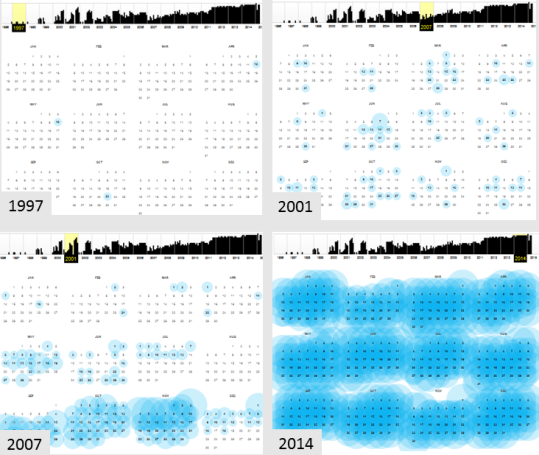
Figure 1: Frequency of whitehouse.gov crawls (selected years)
The most complete .GOV crawls occurred during three month time periods (Nov-Jan) of election years starting in 2004.[9] Using congressional websites URLs as the seeds, the IA captured more government web presence than before. Figure 2 indicates spikes in unique .GOV URLs captured during election years. For example, the number triples from about 500 million to 1.5 billion between 2003 and 2004.
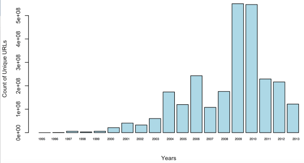
Figure 2: Total .GOV Unique URLs
Although .GOV is less than ideal as a data resource from a conventional social science perspective, there is no other option for investigating two decades of White House website content, or the content of millions of other pages of government website content. Importantly, because these crawls contain snapshots of each page, researchers could hypothetically examine language that agencies or individuals chose to remove – something scraping those same pages now could not provide. The challenge researchers face is finding the hidden gems in a resource that cannot be easily explored.
Big Data and Distributed Computing
.GOV is an excellent platform for learning about “big data” analysis techniques. The basic challenge is that the dataset is too large (90,000 gigabytes) to download and explore. Big data is stored and managed differently. Traditional databases (aka “structured data” are organized into neat rows and columns.[10] Big data projects rely on more flexible data storage processes where portions of the data are distributed across a cluster of computers. Each computer in the cluster is a node, and portions of the data are stored in “buckets” or “bins” within each node (see Figure 3). To access the data, researchers use special software to send simultaneous requests to the different nodes. The piecemeal results of these multiple queries are then recombined into a much smaller, single working file.
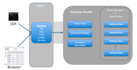
Figure 3: Hadoop System for .GOV
Querying .GOV
The .GOV database is currently hosted on a Hadoop computing cluster operated by a commercial datacloud service, Altiscale (www.altiscale.com). Within the cluster housing .GOV, the data are distributed across nine separate “buckets.” Each bucket contains thousands of large (100mb) WARC (Web Archive Container) files (or `ARC’ files for earlier records). Each of these WARC files then contains thousands of individual webpage capture records. As mentioned, each capture record includes the parsed text, the URLs found on the page, the full content of the capture (including images and video files); and the CDX index file. The CDX file includes useful metadata about specific records that can be used to find and exclude particular records, such as the URL, timestamp, Content Digest, MIME type, HTTP Status Code, and the WARC file where it is located.
The data are accessed using Apache software programs. Apache Pig and Hive are SQL-based languages that can be used for basic data processing such as joining or merging files, searching for specific URLs, and more generally retrieving data of interest. Many Apache commands will be familiar to users with working knowledge of SQL, R or Python. To search all of the capture records in the .GOV database, one must write a query to search thousands WARC files across each of the nine buckets.
Obtaining a key and creating a workbench
Here we describe the big picture process of querying .GOV. In the next section, we present some preliminary findings using the parsed text data. The specific annotated scripts used to accomplish the latter can be found in the online Appendix.
Users must first gain access to the Altiscale computing cluster by requesting an “ssh” key (detailed on Altiscale’s website – you have to email accounts@altiscale.com to request a key). Each key owner is granted a local workbench (an Apache Work Station (AWS)) on the cluster that is similar to the “desktop” of a personal computer and contains the Apache software programs needed to query the database. About 20 gb of storage is also provided (the .GOV database is about 4500 times larger).
Writing scripts to extract information
1. Specifying what is to be collected
Apache Hive and Pig are used execute SQL queries. This can be done on the command line directly (there is no GUI option), but it is easier to write and store scripts on the workbench, and then write a command to execute them across the buckets of interest. For example, one can write an Apache Pig script that requests each parsed text file from a specified URL (e.g. whitehouse.gov), separates the parsed text fields (“date” “URL” “content” “title” etc.), searches each field for each record for a keyword or regular expression, and then counts how many times a match occurs. The full parsed text could also be downloaded in order to explore the content in more detail later. But with so much data (1.1 billion pages), such a collection can quickly become too large to export.
The functionality of Pig and Hive (like SQL) is limited. For example, Pig will return and count the webpage captures that contain a keyword (true/false) for a date range (e.g., per month/year), but it can’t compute the frequency of keyword mentions. To do more detailed or custom analysis, researchers can write user defined functions (UDFs) in Python. The Python script is stored on the workbench as a .py file and then called by the Pig script.[11]
Processing time is a major consideration. Even simple jobs such as keyword counts can take hours or even days to run over so much data. More computationally intensive methods, such as topic models may be impractical. The best way to discover whether a script is going to work and how long it will take is to test it on a subset of the data, such as on just one WARC file in one of the buckets. Running a complete job without testing it is likely to lead to many hours or days of waiting only to discover that it did not work. Linux “Screen” (already installed on the cluster) can then be used to run the script across the cluster remotely (so that your own computer can be used for other things).[12]
2. Providing instructions about where to search on the cluster
The CDX files provide guidance that makes it possible to limit queries to particular URLs, date ranges, WARC files etc.[13] For example, the first query might identify and produce a list of all of the URLs that contain the keyword. The next query would focus on extracting the relevant information (such as keyword and total word counts) from that more limited set of URLs.
3. Concatenating and exporting the results
Query results for each WARC or ARC file (containing thousands of captures) are stored separately on the cluster. Additional scripts must be written to concatenate them. Whether the results can be exported can also be calculated at this point.[14]
Application: Government Attention to the Financial Crisis, Terrorism, and Climate Change
As a starting point to discovering what’s in .GOV, we investigate keyword frequencies for three recent issues in American politics. We hope to observe patterns consistent with what is generally known about the issues, and perhaps more novel patterns that begin to illustrate the potential of this new data source.
Collecting the data
We first created a limited list of top level URLs (departments, agencies and political institutions) relevant to the three issues. For example, the regular expression “.house.gov” theoretically captures every web page of every branch of the official website of the U.S. House of Representatives that the IA collected. This includes, among other things, every Representative’s official website (e.g., pelosi.house.gov) and every House committee’s website (e.g., agriculture.house.gov). Aggregating results during the collection process in this way means that we cannot pull out just the results for a particular member or committee’s website. That would require a different query using more specific URLs.
We then counted keyword mentions on every subpage of that root URL. We first developed broad lists of keywords related to the three issues. After obtaining results, we created more refined lists by dropping terms that seemed problematic or were used less often (see online appendix). For example, we dropped “security” from the terrorism keyword list because it was too general (e.g., financial security). Running the query over all WARC files took about five days of processing time. All together, the results reported below are based on 8.3 billion keyword hits generated by searching about 600 billion words found on the parsed text pages of the specified URLs.
Focusing on raw counts of keywords gives more weight to larger domains. Any changes in attention to terrorism at the much larger State Department will swamp changes at the Bureau of Alcohol, Tobacco and Firearms (ATF). We focus on the proportion of attention given to the issue within an agency or political institution, by dividing the number of keyword hits by total website words. A proportion-based approach also does a better job of controlling for the expanding size of government web presence.
Overall Trends
One way to begin to assess the validity of using website content to study political attention is to ask whether changes in content correlate with known events. For each issue in Figure 4, we identified the URLs (federal government organizations) thought to play a role on the issue (see Appendix II for these lists and URLs). The graphs then report average proportions of attention across these URLs.[15] Attention to terrorism similarly increases after 9/11/2001, but government-wide attention to terrorism increases most dramatically from 2005 to 2006. Institutionalization is almost certainly part of the explanation. We are capturing attention to terrorism (relative to other issues) on the websites of government agencies. The Department of Homeland Security was not created until 2003 and one of the purposes of its creation was to re-orient the missions of existing agencies (such as FEMA) towards preventing and responding to terrorism. In addition, while 9/11 was an important focusing event for the US, terrorism worldwide continued to increase post 9/11. As we might expect, there is no evidence of equivalent shocks for climate change.
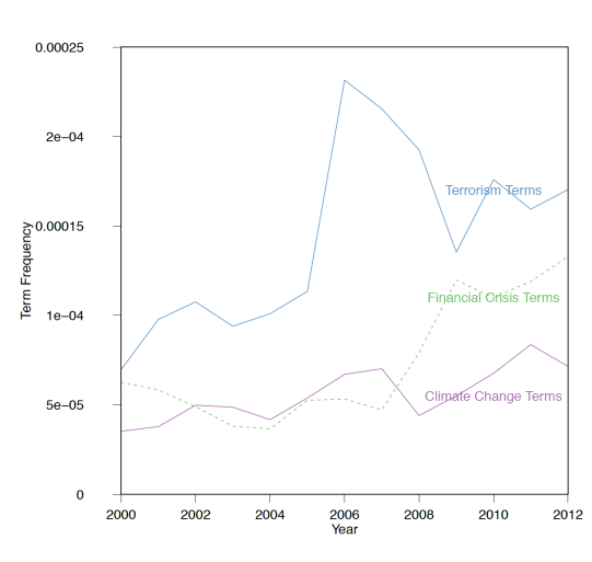
Figure 4: Issue Attention Across .GOV
Diffusion of Attention to Terrorism
Political scientists have long been interested in how “focusing events” impact political attention (Birkland 1998). Many studies have examined the impact of 9/11 on the organization and activities of specific government agencies and departments. Here, we ask how attention to terrorism spread across government departments and agencies. Entropy is a measure disorder that is frequently used to study the dispersion of political attention (Boydstun et al. 2014). Figure 5 confirms that attention to terrorism in the federal government became more dispersed post 9/11.[16]
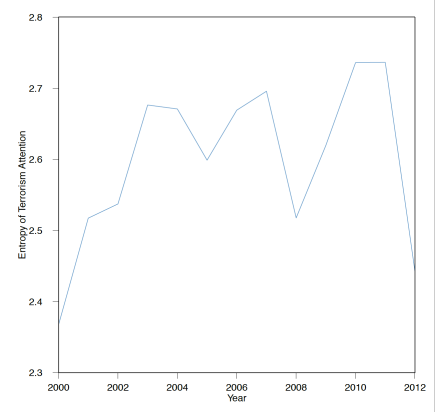
Figure 5: Diffusion in Attention Across .GOV
A Financial “Bubble”?
One of the questions raised in congressional hearings after the 2007-08 financial crisis was whether it could have been anticipated and averted. A related question is whether government agencies saw it coming. As an historical archive, .GOV may provide some clues. Here we simply examine “bubble” mentions across organizations (as a proportion of total website words). Figure 6 indicates that references to bubbles spike in the elected branches after the meltdown, whereas bubble mentions at the four agencies most responsible for the economy increase 2-3 years ahead of the crisis. Bubbles also see increased attention at the Federal Reserve before the stock market sell-off in 2001.
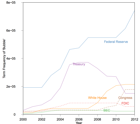
Figure 6: Attention to Financial Crisis Across .GOV
Framing Climate Change
Early in President G.W. Bush’s first term of office, pollster Frank Luntz advised Republicans to talk about “climate change” rather than “global warming” because focus groups saw the latter as more of a threat (Leiserowitz et al. 2014, 7). Subsequent academic research also found that the public is somewhat more likely to support action to address global warming. However, it seems as though conservatives also spend much of their time ridiculing global warming. Recently Senator James Inhofe (R-OK) brought a snowball to the Senate floor to question scientists’ claims that 2016 was one of the warmest years on record (Bump 2015). If conservatives have discredited global warming in the eyes of the public, then proponents of climate action may have less incentive to use that frame.
In Figure 7, values above .50 indicate that climate change mentions are more common than global warming mentions. “Agencies” refers to the average emphasis on climate change for four agencies with central roles (the EPA, NSF, NOAA, and NASA). According to Figure 7, scientific agencies have always emphasized climate change over global warming, with climate change increasingly favored in recent years. For the elected branches, the patterns are more variable and seem to support the notion that conservatives control the global warming frame. In Congress, global warming has been a more popular frame during periods of Republican control (2001-2008; 2011-2013) and has been used more often over time. The patterns for the White House do not support what Luntz advised. Global warming receives more attention than climate change for most of the years of the Bush administration. The Obama administration, in contrast, has gone all in for climate change. Although preliminary, these results do suggest that conservatives have defanged what was once the most effective frame for winning public support for climate action.
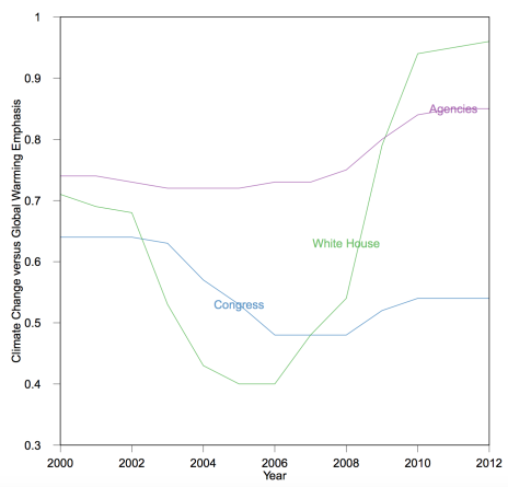
Figure 7: Attention To Climate Change Across .GOV
Conclusion
Accessing this big data resource requires new skills and a new mindset. In terms of skills, we hope that our description of the process and working scripts lower the bar. In terms of mindset, political scientists working with statistical methods are used to immediate results. Exploring .GOV in this way is not an option (the Wayback Machine is probably the best way to get a sense of what’s in .GOV, and it can take days or even weeks to run a query). On the other hand, .GOV contains insights available nowhere else. Although the current database has important limitations, the Internet Archive recently embarked on a collaboration with many partners to scrape all federal government agencies as completely as possible prior the end of the Obama administration. If this effort is successful and if similar efforts follow in subsequent years, .GOV will be an even more valuable resource for investigating a wide range of questions about the federal bureaucracy and federal programs.
Bibliography
“Bash Shell Basic Commands.” GNU Software.
Boydstun, A. E., Bevan, S. and Thomas, H. F. (2014), “The Importance of Attention Diversity and How to Measure It.” Policy Studies Journal, 42: 173–196. doi: 10.1111/psj.12055
Bump, P. “Jim Inhofe’s Snowball Has Disproven Climate Change Once and for All.” The Washington Post, 26 Feb. 2015. Web. 28 June 2016.
Birkland, T. A. (1998). “Focusing events, mobilization, and agenda setting.” Journal of Public Policy. 18(01), 53-74.
Edwards, J., McCurley, K. S., and Tomlin, J. A. (2001). “An adaptive model for optimizing performance of an incremental web crawler”. Tenth Conference on World Wide Web (Hong Kong: Elsevier Science): 106–113.
“The History of the Internet.” The Internet Society.
“The Internet Archive.” Internet Archive. https://archive.org/
Kahn, R. (1972). “Communications Principles for Operating Systems.” Internal BBN memorandum.
Leiner et al. “Brief History of the Internet.”
Leiserowitz, A. WHAT’S IN A NAME? GLOBAL WARMING VERSUS CLIMATE CHANGE. Rep. Yale Project on Climate Change Communication, May 2014. Web. 28 June 2016.
Licklider, J. C. (1963). “Memorandum for members and affiliates of the intergalactic computer network.” M. a. A. ot IC Network (Ed.). Washington DC: KurzweilAI. ne.
Najork, M and J. L. Wiener. (2001). “Breadth-first crawling yields high-quality pages.” Tenth Conference on World Wide Web, (Hong Kong: Elsevier Science): 114–118.
“The Rise of 3G.” THE WORLD IN 2010. International Telecommunication Union (ITU).
Sagiroglu, S., & Sinanc, D. (2013, May). “Big data: A review.” In Collaboration Technologies and Systems (CTS), 2013 International Conference (pp. 42-47). IEEE.
“A “ssh” key (Secure Shell)” (2006).
Vance, A. (2009). “Hadoop, a Free Software Program, Finds Uses Beyond Search”. The New York Times. 27 February 2017.
Appendix I
The following script flags all web pages that include one or more mentions of the term `climate change’ and stores the full text of those captures. We begin with an overview of the process of running jobs on the cluster, and then provide specific code. For questions, please contact the authors.
Overview
Running scripts on the cluster requires a basic understanding of bash (Unix) shell commands using the Command Line on a home computer (on a Mac, this is the program “Terminal”). For a basic rundown of bash commands, see here.
Begin by opening a bash shell on a home desktop, and using an ssh key obtained from Altiscale to login. Once logged in, you will be on your personal workbench and now have to use a script editor (such as Vi). Come up with a name for the script, open the editor, and then either paste or write the desired script in the editor, close and save the file (to your personal workbench on the cluster).
Scripts must be written in Hadoop-accessible languages, such as Apache Pig, Hive, Giraph or Oozie. Apache languages are SQL-like, which means if you have experience with SQL, MySQL, SQLlite or PostgreSQL (or R or Python), the jump should not be too big. For text processing, Apache Pig is most appropriate, whereas for link analysis, Hive is best. The script below is written in Apache Pig and a manual can be found at https://pig.apache.org/. For an example of some scripts written for this cluster, see here. May be easiest to it “clone” the “archive analysis” file hosted on GitHub from Vinay Goel or three basic scripts from Emily Gade .govDataAnalysis and use those as a launchpoint. If you don’t know how to use GitHub, see here.
Because Apache languages have limited functionality, users may want to write user defined functions in a program like Python. A tutorial about how to do this can be found here.
Once a script is written, you will want to run it on a segment of the cluster. This requires another set of Unix style Hadoop shell commands. Users must then specify the file path(s), the desired output directory, and where the script can be found.
Getting a Key
As discussed above, this script is run from your workbench on the cluster. To gain access, you will need to set up an SSH “key” with Altiscale. Once you have obtained and sent your SSH key to Alitscale, you can log in using any bash shell from your desktop with the command “ssh altiscale”.
Locating the Data
The Altiscale cluster houses 9 “buckets” of .GOV data. Each bucket contains hundreds or thousands of Web Archive Files (older version are “ARC” files, newer version are “WARC” files, but they have all the same fields). Each WARC/ARC file contains captures from the same crawl, but it (a) won’t contain all of the captures from a given crawl, and (b) since the crawl is doing a lot of things simultaneously, captures of a single site can be located in different WARC files.
With so much data, there is no simple “table” or directory that can be consulted to locate a specific web page. The best way to find specific pages is to use Hive to query the CDX database. See Vinay Goel’s GitHub for details about how to query CDX. If a user knows exactly what he or she wants (all the captures of the whitehouse.gov main page, or all the captures from September 11, 2001), the CDX can tell you where to find them. Otherwise, users will want to query all of the buckets because there is no easy way to learn where results are stored. (Though we advise first testing scripts on a single bucket or WARC file.)
First, use the command line with SSH interface to query the data directories and see which buckets or files to run a job over. This requires the Hadoop syntax to “talk” to the cluster where all the data is stored. The cluster has a user-specific directory where users can store the results of scrapes. A user’s local workbench does not have enough space to save them.
Whenever users “talk” from a user’s local workbench to the main cluster, users need to use `hadoop fs -‘ and then the bash shell command of interest. For a list of Hadoop-friendly bash shell commands, see here.
For example, the line of code
hadoop fs -ls
pulls a listing of the files in your personal saved portion of the cluster (in addition to the local workbench, each user has a file directory to save the results). As well,
hadoop fs -ls /dataset-derived/gov/parsed/arcs/bucket-2/
would draw up all the files in Bucket #2 of the parsed text ARCS directory.
Defining Search Terms
Scripts that deal with text are best written in Apache Pig. Hadoop also supports Apache Hive, Giraffe and Spark. To find and collect terms or URLs of interest, users will need to write a script. For example, users might write a script to flag any captures that have a mention of a global warming term, and return the date of the capture, URL, page title, checksum, and the parsed text. This script is saved on your local workbench and needs to have a .pig suffix. Users will need to use some sort of bash editor to write and store the script such as vi (details about how to use vi can be found above). Script is below. The first four lines are defaults and also set the memory.
Script begins:
SET default_parallel 100;
SET mapreduce.map.memory.mb 8192;
SET mapred.max.map.failures.percent 10;
REGISTER lib/ia-porky-jar-with-dependencies.jar;
DEFINE FROMJSON org.archive.porky.FromJSON();
DEFINE SequenceFileLoader org.archive.porky.SequenceFileLoader();
DEFINE SURTURL org.archive.porky.SurtUrlKey();
The sequence file loader pulls the files out of the ARC/WARC format and makes them readable. Note, when they were put into the ARC/WARC format, they were run through a HTML parser to remove the HTML boilerplate. However, if the file was not in HTML to begin with, the parser will just produce symbols and this won’t fix it. Users will have to deal with those issues separately.
When loading data on the command line (instructions below), give the data a name (here $I_Parsed_Data) and make sure to use the same “name” for the data in the command line command. This is a stand-in for the name of the directory or file over which you will run a script.
Archive = LOAD "$I_PARSED_DATA" USING SequenceFileLoader()
AS (key:chararray, value:chararray);
Archive = FOREACH Archive GENERATE FROMJSON(value) AS m:[];
Archive = FILTER Archive BY m#`errorMessage' is null;
ExtractedCounts = FOREACH Archive GENERATE m#`url' AS src:chararray,
   SURTURL(m#`url') AS surt:chararray,
   REPLACE(m#`digest',`sha1:','') AS checksum:chararray,
   SUBSTRING(m#`date', 0, 8) AS date:chararray,
   REPLACE(m#`code', `[^p{Graph]', ` ') AS code:chararray,
   REPLACE(m#`title', `[^p{Graph]', ` ') AS title:chararray,
   REPLACE(m#`description', `[^p{Graph]', ` ')AS description:chararray,
   REPLACE(m#`content', `[^p{Graph]', ` ') AS content:chararray;
The above code block says: for each value and key pair, pull out the following fields. Chararray means character array – so a list of characters with no limits on what sort of content may be included in that field. The next line selects the first eight characters of the date string (year, month, day). The full format is year, month, day, hour, second. Unicode errors can wreck havoc on script and outputs. The regular expression p{Graph means “all printed characters”– e.g., NOT newlines, carriage returns, etc. So, this query finds anything that is not text, punctuation and whitespace, and replaces it with a space. Also note that because Pig is under-written in Java, users need two escape characters in these scripts (whereas only one is needed in Python).
UniqueCaptures = FILTER ExtractedCounts BY content MATCHES
`.*naturals+disaster.*' OR content MATCHES `.*naturals+disaster.*'
OR content MATCHES `.*desertification.*' OR content MATCHES
`.*climates+change.*' OR content MATCHES `.*pollution.*' OR
content MATCHES `.*foods+security.*';
This filters out the pages with keywords of interest (in this case words related to climate change) and keeps only those pages.
STORE UniqueCaptures INTO `$O_DATA_DIR' USING PigStorage('\u0001');
This stores the counts the file name given to it.
The “using PigStorage” function allows users to set their own delimiters. I chose a Unicode delimiter because commas/tabs show up in the existing text. And, since I stripped out all Unicode above, this should be clearly a new field. Save this script to your local workbench.
Another option would be to count all the mentions of specific terms. Instead of the above, users would run:
SET default_parallel 100;
SET mapreduce.map.memory.mb 8192;
SET mapred.max.map.failures.percent 10;
REGISTER lib/ia-porky-jar-with-dependencies.jar;
This line allows you to load user-defined functions from a Python file:
REGISTER `UDFs.py' USING jython AS myfuncs;
DEFINE FROMJSON org.archive.porky.FromJSON();
DEFINE SequenceFileLoader org.archive.porky.SequenceFileLoader();
DEFINE SURTURL org.archive.porky.SurtUrlKey();
Archive = LOAD `$I_PARSED_DATA' USING SequenceFileLoader()
AS (key:chararray, value:chararray);
Archive = FOREACH Archive GENERATE FROMJSON(value) AS m:[];
Archive = FILTER Archive BY m#`errorMessage' is null;
ExtractedCounts = FOREACH Archive GENERATE m#`url' AS src:chararray,
   SURTURL(m#`url') AS surt:chararray,
   REPLACE(m#`digest',`sha1:',`') AS checksum:chararray,
   SUBSTRING(m#`date', 0, 8) AS date:chararray,
   REPLACE(m#`code', `[^p{Graph]', ` ') AS code:chararray,
   REPLACE(m#`title', `[^p{Graph]', ` ') AS title:chararray,
   REPLACE(m#`description', `[^p{Graph]', ` ')AS description:chararray,
   REPLACE(m#`content', `[^p{Graph]', ` ') AS content:chararray;
If a user has function which selects certain URLs of interest and groups all other URLs as “other”, they would run it only on the URL field. And, if a user has a function that collects words of interest and counts them as well as total words, the user should run that through the content field. Code for using those UDFs would look something like this:
UniqueCaptures = FOREACH ExtractedCounts GENERATE myfuncs.pickURLs(src),
   src AS src,
   surt AS surt,
   checksum AS checksum,
   date AS date,
   myfuncs.Threat_countWords(content);
In Pig, and the default delimiter is `\n’ (new line) but many `\n’ appear in text. So one must get rid of all the new lines in the text. This will affect our ability to do text parsing by paragraph, but sentences will still be possible. Code to get rid of the `\n’ (new line delimiters) which are causing problems with reading in tables might look something like this:
UniqueCaptures = FOREACH UniqueCaptures GENERATE REPLACE(content, `\n', ` ');
To get TOTAL number of counts of web pages, rather than simply unique observations, merge with checksum data:
Checksum = LOAD `$I_CHECKSUM_DATA' USING PigStorage() AS (surt:chararray,
date:chararray, checksum:chararray);
CountsJoinChecksum = JOIN UniqueCaptures BY (surt, checksum),
Checksum BY (surt, checksum);
FullCounts = FOREACH CountsJoinChecksum GENERATE
   UniqueCaptures::src as src,
   Checksum::date as date,
   UniqueCaptures::counts as counts,
   UniqueCaptures::URLs as URLs;
This would sort counts by original “source” or URL:
GroupedCounts = GROUP FullCounts BY src;
This fills in the missing counts and stores results:
GroupedCounts = FOREACH GroupedCounts GENERATE
   group AS src,
   FLATTEN(myfuncs.fillInCounts(FullCounts)) AS (year:int,
   month:int, word:chararray, count:int, filled:int,
   afterlast:int, URLs:chararray);
STORE GroupedCounts INTO `$O_DATA_DIR';
The UDFs mention here (pickURLs, Threat_countWords, and FillinCounts) are written in Python and can be seen in at the bottom of this Appendix.
Running the Script
To run this script, type the following code into the command line, after having logged in the Altiscale cluster with your ssh key. Users will select the file or bucket they want to run the script over, and type in an “output” directory (this will appear on your home/saved data on the cluster, not on your local workbench). Finally, users need to tell Hadoop which script they want to run. The I_PARSED_DATA was defined as the location of the data to run the script over in the script above. Here we telling the computer that this bucket is the I_PARSED_DATA. Next, one must load the CHECKSUM data, and finally, give the output directory, and the location of your script.
The following should be run all as one line:
pig -p I_PARSED_DATA=/dataset-derived/gov/parsed/arcs/bucket-2/ -p I_CHECKSUM_DATA=/dataset/gov/url-ts-checksum/ -p O_DATA_DIR=place_where_you_want_the_file_to_end_up location_of_your_script/scriptname.pig
Exporting Results
Lastly, to remove results from the cluster users need to open a new Unix shell on their local machine that is NOT logged in to the cluster with their ssh key. Then type the location of the file they’d like to copy and give it a file path for where they’d like to put it on their desktop. For example:
The following should be run all as one line:
scp -r altiscale:~/results_location/location_on_your_computer_you_want_to_move_results_to/
Python UDFs
#import packages
from collections import defaultdict
import sys
import re
#define output schema so the UDF can talk to Pig
@outputSchema("URLs:chararray")
# define Function
def pickURLs(url):
   try:
   # these can be any regular expressions
     keyURLs = [
     `state\.gov',
     `treasury\.gov',
     `defense\.gov',
     `dod\.gov',
     `\.house\.gov']
     URLs = []
     for i in range(len(keyURLs)):
        tmp = len(re.findall(keyURLs[i], url, re.IGNORECASE))
         if tmp > 0:
          return keyURLs[i]
     return `other'

# counting words
#define output schema as a "bag" with the word and then the count of the word
@outputSchema("counts:bag{tuple(word:chararray,count:int)")
def Threat_countWords(content):
   try:
     # these can be any regular expressions
     Threat_Words = [
           `(natural\sdisaster)',
           `(global\swarming)',
           `pollution',
           `(climate\schange)']
#if you want a total of each URL or page, include a total count
     threat_counts = defaultdict(int)
     threat_counts[`total'] = 0
     if not content or not isinstance(content, unicode):
        return [((`total'), 0)]
     threat_counts[`total'] = len(content.split())
     for i in range(len(Threat_Words)):
        tmp = len(re.findall(Threat_Words[i], content, re.IGNORECASE))
         if tmp > 0:
          threat_counts[Threat_Words[i]] = tmp
    # Convert counts to bag
     countBag = []
     for word in threat_counts.keys():
         countBag.append( (word, threat_counts[word] ) )
     return countBag

## filling in counts using CHECKSUM and carrying over counts
from the "last seen" count
@outputSchema("counts:bag{tuple(year:int, month:int, word:chararray, count:int,filled:int, afterLast:int, URLs:chararray)")
def fillInCounts(data):
   try:
     outBag = []
     firstYear = 2013
     firstMonth = 9
     lastYear = 0
     lastMonth = 0
# used to compute averages for months with multiple captures
# word -> (year, month) -> count
     counts = defaultdict(lambda : defaultdict(list))
     lastCaptureOfMonth = defaultdict(int)
     endOfMonthCounts = defaultdict(lambda : defaultdict(lambda:
     dict({`date':0,`count':0)))
     seenDates = {
#ask for max observed date
     for (src, date, wordCounts, urls) in data:
         for (word, countTmp) in wordCounts:
           year = int(date[0:4])
           month = int(date[4:6])
           if isinstance(countTmp,str) or isinstance(countTmp,int):
               count = int(countTmp)
           else:
               continue
           ymtup = (year, month)
           counts[word][ymtup].append(count)
           if date > lastCaptureOfMonth[ymtup]:
              lastCaptureOfMonth[ymtup] = date
           if date > endOfMonthCounts[word][ymtup]['date']:
               endOfMonthCounts[word][ymtup]['date'] = date
               endOfMonthCounts[word][ymtup]['count'] = count
           seenDates[(year,month)] = True
           if year  lastYear:
               lastYear = year
               lastMonth = month
           elif year == lastYear and month > lastMonth:
               lastMonth = month
     for word in counts.keys():
# The data was collected until Sep 2013
# make sure that you aren't continuing into the future
         years = range(firstYear, 2014)
         useCount = 0
         afterLast = False
         filled = False
         ymLastUsed = (0,0)
         for y in years:
           if y > lastYear:
               afterLast = True
           if y == firstYear:
               mStart = firstMonth
           else:
               mStart = 1
           if y == 2013:
               mEnd = 9
           else:
               mEnd = 12
           for m in range(mStart, mEnd+1):
              if y == lastYear and m > lastMonth:
                 pass
              if (y,m) in seenDates:
# Output sum, as we will divide by sum of totals later
                 useCount = sum(counts[word][(y,m)])
                 ymLastUsed = (y,m)
                 filled = False
              else:
# If we didn't see this date in the capture, we want to use the last capture we saw
# previously (we might have two captures in Feb, so for Feb we output both,
# but to fill-in for March we would only output the final Feb count)
# Automatically output an assumed total for each month (other words
# may no longer exist)
                 if endOfMonthCounts[word][ymLastUsed]['date'] ==                 lastCaptureOfMonth[ymLastUsed]:
                     useCount = endOfMonthCounts[word][ymLastUsed]['count']
                 else:
                     continue
                 filled = True
              if useCount == 0:
                 continue
              outBag.append((y, m, word, useCount, int(filled), int(afterLast), urls))
Appendix II: Lists of URLs and Terms
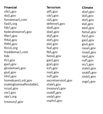
Figure 8: URLs used for this study
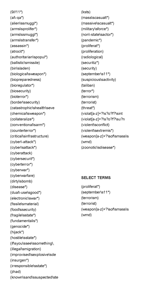
Figure 9: Terrorism Terms
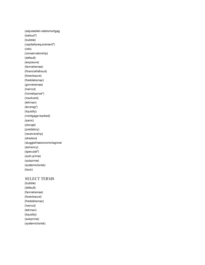
Figure 10: Finance Terms
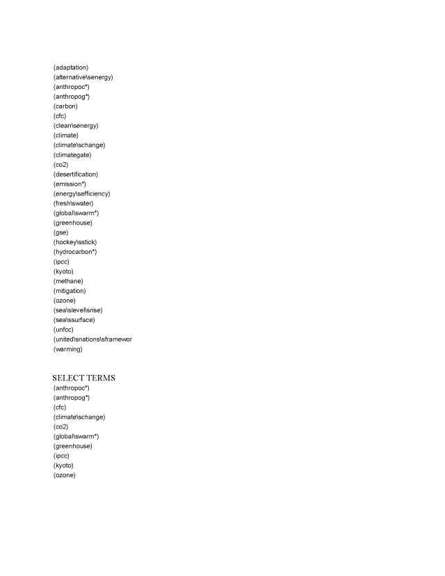
Figure 11: Climate Terms
Notes
[1] For example, see this article on understanding Big Data: Sagiroglu, S., & Sinanc, D. (2013, May). Big data: A review. In Collaboration Technologies and Systems (CTS), 2013 International Conference (pp. 42-47). IEEE.
[2] In thinking about using the volume of the Library of Congress as a unit of measure, see: “A “Library of Congress” Worth of Data” by Leslie Johnston, April 25, 2012.
[4] See the Internet Archive’s description of their sub-collections here.
[5] .GOV also includes state and local websites that use the .gov suffix. Whereas the Wayback Machine makes it possible to view date-specific individual websites, the .GOV collection can be used to investigate patterns across websites and over time.
[6] See Google’s Official Blog (July 25, 2008) for discussion at “We knew the web was big…”
[7] These are listed in the online Appendix.
[8] The graphs are copied from Wayback Machine search results for whitehouse.gov.
[9] According to Vinay Goel, senior data engineer at the IA, the Library of Congress contracted with the IA to systematically capture congressional websites during these time periods.
[10] See Sagiroglu & Sinanc
[11] See Pig Wiki and Pig manuel.
[12] For instructions about how to use Screen see here.
[13] Instructions for querying the CDX file can be found here. For queries than cannot be restricted in advance (e.g. the research objective is to identify all parsed text files that contain a particular keyword), breaking a job into steps can be more efficient.
[14] Instructions for exporting documents from the Altiscale cluster can be found here. If they cannot, Apache Giraffe is designed to facilitate analyses and graphing on the cluster.
[15] The different proportions for the different issues are not comparable because they are dependent on the keyword lists. Financial crisis term usage (as a proportion of all terms) spikes upward in 2007-08 as expected (and also in 2001 when there was another stock market decline).
[16] Our measure is based on the proportion of domain content for 23 departments and agencies, where entropy is based on each domain’s proportion of the sum of all agencies’ proportions.