By Benjamin Ferland [1]
Since Brambor, Clark and Golder’s (2006) article in Political Analysis (hereafter BCG), our understanding of interaction models has improved significantly and most empirical scholars have now integrated the tools to execute and interpret interaction models properly. In particular, one of the main recommendations of BCG was to include all constitutive terms of the interaction in the model specification. However, BCG acknowledge (in the text surrounding equation 7 of their paper) that there is a mathematically equivalent model specification that allows researchers to exclude certain constitutive terms from an interaction model when one of the modifying variables is discrete. A recent review experience made me realize that this exception is not as widely recognized as BCG’s core advice to include all constitutive terms, suggesting therefore, that a brief note to the scholarly community might be important in publicizing this exception. In the next section, I show the equivalency of BCG standard specification and this alternative specification. I then provide a brief example of both approaches when applied in a substantive case — Adams et al. (2006) study “Are Niche Parties Fundamentally Different from Mainstream Parties?” — and show that we get the same results either using BCG’s approach or the alternative approach.
Overall, I show that while the two model specifications are equivalent, each has some advantages in terms of the interpretation of the regression results. On the one hand, the advantage of the standard specification is to present directly in the regression results whether the difference in the marginal effects of X on Y between the categories of the modifying variable Z is statistically significant. On the other hand, the main benefit of the alternative approach is to present directly in the regression results the marginal effects of X under each category of the modifying variable Z. Researchers may thus choose between the two equivalent specifications depending on the results they want to present and emphasize.
1 Equivalency of the Standard and Alternative Specifications
In order to show the equivalency of BCG standard specification and the alternative specification when one of the modifying variables is discrete, I take as an example a dependent variable Y which is a function of an interaction effect between a continuous variable X and a dummy variable D. BCG standard approach to interaction models indicates that we must multiply the variables X and D and include this interaction term as well as the constitutive terms X and D, respectively, in the regression model. Specifically, the standard specification is the following:
Y = b0 + b1D + b2X + b3XD + ϵ (1)
where X is continuous and D is a dummy variable (0,1). The marginal effect of X when D = 0 is given by b2 while the marginal effect of X when D = 1 is given by b2 + b3.[2]
The alternative approach explained briefly in BCG (see equation 7) and Wright (1976) consists in treating the dummy variable D as two dummy variables: D, the original variable, which equals 0 and 1 and D0, the inverse of D, which equals 1 when D = 0 and 0 when D = 1. For example, if D is a dummy variable where 1 represents democratic countries and 0 authoritarian countries D0 would simply be the inverse dummy variable where 1 represents authoritarian countries and 0 democratic countries. Consequently, D + D0 = 1 and D0 = 1 − D. The alternative approach consists in multiplying X respectively with D and D0, including all constitutive terms in the regression model except X and one of the dummy variables, D or D0. The reason for including only D or D0 is that these variables are perfectly collinear. It is not possible to include X neither because of perfect multicollinearity with XD and XD0.
The alternative specification is thus the following:
Y = a0 + a1D + a2XD + a3XD0 + ϵ (2)
Equation 2 could be rewritten as
Y = a0 + a1D + a2XD + a3X(1 − D) + ϵ (3)
Equation 3 highlights explicitly that we do not necessarily need to create D0 but only to multiply X by (1 − D). In equations 2 and 3, the marginal effect of X when D = 0 (i.e. when D0 = 1) is given by a3 while the marginal effect of X when D = 1 is given by a2.[3]
The main advantage of this alternative specification is that for each category of the discrete modifying variable D (0 and 1 in this case) the marginal effect of X and its associated standard error are provided directly from the regression results. This is not the case in the standard approach where only one of these results is directly provided (i.e. b2, the effect of X when D=0). Consequently, we need to add up b2 and b3 to obtain the effect of X when D=1. This is easy to do in Stata with the command lincom (lincom _b[coef ] + _b[coef ]).
A disadvantage of the alternative specification is that the regression results do not indicate whether the difference between the marginal effects of X when D=0 and when D=1 is statistically significant. This is the advantage of the standard approach which provides this information in the regression results . If the coefficient b3 is statistically significant in equation 1, this indicates that the marginal effect of X when D=1 is statistically different than the marginal effect of X when D=0. To answer this question with the alternative approach, we must test the equality of a2 and a3. This is also straightforward in Stata with the command test (test _b[coef ] = _b[coef ]) or lincom (lincom _b[coef ] − _b[coef ]).
The specification of the alternative approach could be easily generalized to discrete variables with multiple categories whether the discrete variable is nominal or ordinal. The procedure is the same. We need first to create a dummy variable for each category of the discrete modifying variable. We then multiply X with each of these dummy variables and include all constitutive terms in the equation (except X and one of the dummy variables). This specification will also allow researchers to evaluate directly the magnitude of the substantive effect of X across the different values of the discrete modifying variables without including all constitutive terms of the interaction explicitly.
2 Replication of “Are Niche Parties Fundamentally Different From Mainstream Parties?”
In this section, I compare the results of the standard and alternative approaches to interaction models in replicating Adams et al. (2006) study “Are Niche Parties Fundamentally Different from Mainstream Parties?” published in the American Journal of Political Science. Two main research questions are examined in this article. First, the authors examined whether mainstream parties are more responsive than niche parties to shift in public opinion in adjusting their policy programs. Second, and building on this prediction, they examined whether niche parties are more penalized electorally than mainstream parties when they moderate their policy positions. Here, I only replicate their model associated with the first question.
Adams et al. (2006) tested these hypotheses in seven advanced democracies (Italy, Britain, Greece, Luxembourg, Denmark, Netherlands, and Spain) over the 1976-1998 period. They measure parties’ policy position on the left-right ideological scale with data from the Comparative Manifesto Project (CMP). Surveys from the Eurobarometer are used to locate respondents on the corresponding left-right ideological dimension. Public opinion is measured as the average of all respondents’ self-placement. Finally, the authors coded Communist, Green, and Nationalist parties as niche parties with a dummy variable.
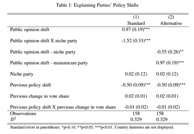
In table 1, I examine party responsiveness to public opinion and present the results of the standard and alternative approaches. Adams et al. (2006) use the standard approach and interact the variable public opinion shift with the dummy variable niche party. The dependent variable is the change in a party’s left- right position. Adams et al. (2006) thus specified a dynamic model where they assess whether a change in public opinion influences a change in party positions between two elections. The models include fixed effects for countries and a number of control variables (see the original study for the justifications). The specification of the standard approach in column (1) is the following:
∆party position = b0 + b1∆public opinion + b2niche party + b3(∆public opinionXniche party) + controls
In column (1) of Table 1, I display the same results as those published in Table 1 of Adams et al. (2006) article. The results in column (1) support the authors’ argument that niche parties are less responsive than mainstream parties to change in public opinion. The coefficient of public opinion shift (0.97) is positive and statistically significant indicating that when public opinion is moving to the left (right) mainstream parties (niche party=0) adjust their policy positions accordingly to the left (right). The coefficient of public opinion shift X niche party indicates that niche parties are less responsive than mainstream parties to shift in public opinion by -1.52 points on the left-right scale and the difference is statistically significant (p
In column (2) of Table 1, I display the results of the alternative approach. The specification is now the following:
∆party position = b0 +b1niche party+b2(∆public opinionXniche party)+b3(∆public opinionXmainstream party)+controls
where mainstream party equals (1 − niche party).
It is important to highlight that the results in columns (1) and (2) are mathematically equivalent. For example, the coefficients of the control variables are exactly the same in both columns. There are some differences, however, in terms of the interpretation of the interaction effect. In column (2), the coefficient of public opinion shift – mainstream party (0.97) equals the coefficient of public opinion shift in column (1). This is because public opinion shift – mainstream party in column (2) indicates the impact of a change in public opinion on the positions of mainstream parties as it is for public opinion shift in column (1). On the other hand, the coefficient of public opinion shift – niche party in column (2) equals -0.55 and is statistically significant at the 0.05 level. This indicates that when public opinion is moving to the left (right) niche parties adjust their policy positions in the opposite direction to the right (left). This result is not explicitly displayed in column (1) when using the standard approach. The coefficient of public opinion shift – niche party in column (2) equals actually the sum of the coefficients of public opinion shift and public opinion shift X niche party in column (1) — i.e. 0.97 + -1.52 = -0.55. In column (2), a Wald-test indicates that the difference of the effects of public opinion shift – niche party and public opinion shift – mainstream party is statistically significant at the 0.01 level, exactly as indicated by the coefficient of public opinion shift X niche party in column (1).
Overall, researchers may choose between two equivalent specifications when one of the modifying variables is discrete in an interaction model: BCG specification which includes all constitutive terms of the interaction and an alternative specification that does not include all constitutive terms of the interaction explicitly. Each specification has its advantages in terms of the interpretation of the interaction effect. The advantage of the alternative approach is to present directly the marginal effects of an independent variable X on Y for each category of the discrete modifying variable Z. On the other hand, the advantage of BCG approach is to present directly whether the difference in the marginal effects of X on Y between the categories of Z is statistically significant. In both specifications, researchers then need to perform an additional test to verify whether the difference in the marginal effects is statistically significant (in the alternative specification) or to calculate the substantive marginal effects under each category of the discrete modifying variable (in the standard specification).
Notes
- Assistant Professor, School of Political Studies, University of Ottawa, 120 University, Ottawa, ON, K1N 6N5, Canada (bferland@uottawa.ca). I thank James Adams, Michael Clark, Lawrence Ezrow, and Garrett Glasgow for sharing their data. I also thank Justin Esarey for his helpful comments on the paper.
- The marginal effect of X in equation 1 is given by b2 + b3D.
- The marginal effect of X in equations 2 and 3 is calculated by a2D + a3D0.
Note also that equation 1 on the left-hand side equals either equation 2 or 3 on the right-hand side:
b0 + b1D + b2X + b3XD + ϵ=a0 + a1D + a2XD + a3X(1 − D) + ϵ
b0 + b1D + b2X + b3XD + ϵ=a0 + a1D + a2XD + a3X − a3XD + ϵ
It is possible then to isolate XD on the right-hand side:
b0 + b1D + b2X + b3XD + ϵ=a0 + a1D + a3X + (a2 − a3)XD + ϵ
Assuming that the models on the left-hand side and right-hand side are estimated with the same data b0 would equal a0, b1 would equal a1, b2 would equal a3 (i.e. the estimated parameter of X(1-D)), and b3 would equal (a2 − a3).
References
Adams, James, Michael Clark, Lawrence Ezrow and Garrett Glasgow. 2006. “Are Niche Parties Fundamentally Different from Mainstream Parties? The Causes and the Electoral Consequences of Western European Parties’ Policy Shifts, 1976-1998.” American Journal of Political Science 50(3):513–529.
Brambor, Thomas, William Roberts Clark and Matt Golder. 2006. “Understanding Interaction Models: Improving Empirical Analyses.” Political Analysis 14:63–82.
Wright, Gerald C. 1976. “Linear Models for Evaluating Conditional Relationships.” American Journal of Political Science 2:349–373.